Phylogenetics
Last updated on 2026-03-31 | Edit this page
Estimated time: 180 minutes
Overview
Questions
- How do you build a simple, distance-based phylogenetic tree?
- How do you build a phylogenetic tree with more advanced methods?
- How do you ascertain statistical support for phylogenetic trees?
Objectives
- Learn the basic of phylogenetics tree building, taking the simplest of the examples with a UPGMA tree.
- Learn how to use phylogenetics algorithms, neighbor-joining and maximum-likelihood.
- Learn how to perform and show bootstraps.
Exercise 1: Paper-and-pen phylogenetic tree
Setup
The exercise is done for a large part with pen and paper, and then a
demonstration in R on your laptop, using RStudio. We’ll also use the R
package ape, which
you should install if it’s not present on your setup. Commands can be
typed or pasted in the “Console” part of RStudio.
R
install.packages('ape')
OUTPUT
- Querying repositories for available source packages ... Done!
The following package(s) will be installed:
- ape [5.8-1]
These packages will be installed into "~/work/course-microbial-genomics/course-microbial-genomics/renv/profiles/lesson-requirements/renv/library/linux-ubuntu-jammy/R-4.5/x86_64-pc-linux-gnu".

# Installing packages --------------------------------------------------------
[32m✔[0m ape 5.8-1                                [linked from cache]
Successfully installed 1 package in 3.1 milliseconds.
And to load it:
R
library(ape)
UPGMA-based tree
Load the tree in fasta format, reading from a temp
file
R
FASTAfile <- tempfile("aln", fileext = ".fasta")
cat(">A", "----ATCCGCTGATCGGCTG----",
    ">B", "GCTGATCCGTTGATCGG-------",
    ">C", "----ATCTGCTCATCGGCT-----",
    ">D", "----ATTCGCTGAACTGCTGGCTG",
    file = FASTAfile, sep = "\n")
aln <- read.dna(FASTAfile, format = "fasta")
Now look at the alignment. Notice there are gaps, which we don’t want in this example. We also remove the non-informative (identical) columns.
R
alview(aln)
OUTPUT
  000000000111111111122222
  123456789012345678901234
A ----ATCCGCTGATCGGCTG----
B GCTG.....T.......---....
C .......T...C.......-....
D ......T......A.T....GCTG
R
aln_filtered <- aln[,c(7,8,10,12,14,16)]
alview(aln_filtered)
OUTPUT
  123456
A CCCGTG
B ..T...
C .T.C..
D T...AT
Now we have a simple alignment as in the lecture. Dots
(.) mean that the sequence is identical to the top row,
which makes it easier to calculate distances.
Calculating distance “by hand”
Let’s use a matrix to calculate distances between sequences. We’ll just count the number of differences between the sequences. We’ll then group the two closest sequences. Which are they?
| A | B | C | D | |
|---|---|---|---|---|
| A | ||||
| B | ||||
| C | ||||
| D |
Here is the solution:
| A | B | C | D | |
|---|---|---|---|---|
| A | ||||
| B | 1 | |||
| C | 2 | 3 | ||
| D | 3 | 4 | 5 |
The two closest sequences are A and B.
Calculating distance “by hand” (continued)
Let’s now cluster together A and B, and calculate the average distance from AB to the other sequences, weighted by the size of the clusters.
| AB | C | D | |
|---|---|---|---|
| AB | |||
| C | |||
| D |
The average distance for AB to C is calculated as follow:
\(d(AB,C) = \dfrac{d(A,C) + d(B,C)}{2} = \dfrac{2 + 3}{2} = 2.5\)
And so on for the other distances:
| AB | C | D | |
|---|---|---|---|
| AB | |||
| C | 2.5 | ||
| D | 3.5 | 5 |
Calculating distance “by hand” (continued)
Now the shortest distance is AB to C. Let’s recalculate the distance to D again.
| ABC | D | |
|---|---|---|
| ABC | ||
| D |
\(d(ABC,D) = \dfrac{d(AB,D) * 2 + d(C,D) * 1}{2 + 1} = \dfrac{3.5 * 2 + 5 * 1}{3} = 4\)
| ABC | D | |
|---|---|---|
| ABC | ||
| D | 4 |
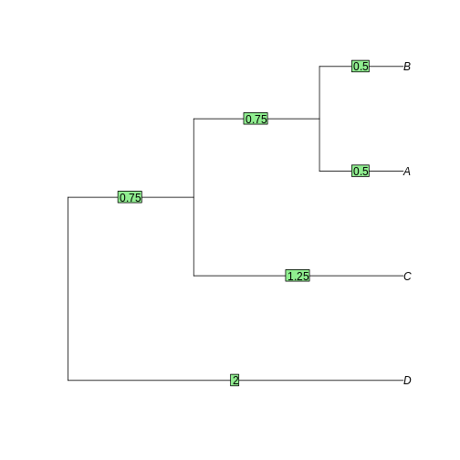
The tree is reconstructed by dividing the distances equally between the two leaves. - A-B: each 0.5. - AB-C: each side gets 2.5/2 = 1.25. The branch to AB is 1.25 - 0.5 = 0.75 - ABC-D: each side gets 4/2 = 2. The branch to ABC is 2 - 0.75 - 0.5 = 0.75

Let’s know do the same using bioinformatics tools.
Challenge
We’ll use dist.dna to calculate the distances. We’ll use
a “N” model, that just counts the differences and doesn’t correct or
normalizes. We’ll use the function hclust to perform the
UPGMA method calculation. The tree is then plotted, and the branch
lengths plotted with edgelabels:
R
dist_matrix <- dist.dna(aln_filtered, model="N")
dist_matrix
OUTPUT
  A B C
B 1
C 2 3
D 3 4 5
R
tree <- as.phylo(hclust(dist_matrix, "average"))
plot(tree)
edgelabels(tree$edge.length)
Exercise 2: Neighbor-joining and Maximum-likelihood tree
Introduction
In the previous episode, we inferred a simple phylogenetic tree using UPGMA, without correcting the distance matrix for multiple substitutions. UPGMA has many shortcomings, and gets worse as distance increases. Here we’ll test Neighbor-Joining, which is also a distance-based, and a maximum-likelihood based approach with IQ-TREE.
Neighbor-joining
The principle of Neighbor-joining method (NJ) is to start from a star-like tree, find the two branches that, if joined, minimize the total tree length, join then, and repeat with the joined branches and the rest of the branches.
Challenge
To perform NJ on our sequences, we’ll use the function inbuilt in
Seaview. First (re-)open the alignment we obtained from
mafft with the E-INS-i method, trimmed with ClipKIT. If it
is not on your computer anymore, transfer it again from Uppmax using
scp or SFTP.
If Seaview is not installed on your computer, download it and install it on your computer.
Challenge (continued)
In the Seaview window, select Trees -> Distance methods. Keep the BioNJ option ticked. BioNJ is an updated version of NJ, more accurate for longer distances. Tick the “Bootstrap” option and leave it at 100. We’ll discuss these later. Then click on “Go”.
What do you see? Is the tree rooted? Is the pattern species coherent with what you know of the tree of life? Any weird results?
Challenge
Redo the BioNJ tree for the other alignment we inferred.
Do you see any differences between the two trees? What can you make out of it?
Maximum likelihood
We will now use IQ-TREE to infer a maximum-likelihood (ML) tree of
the RpoB dataset we aligned with mafft previously. While
you performed the first trees on your laptop, you will infer the ML tree
on Uppmax. As usual, use the interactive command to gain
access to compute time. Go to the phylogenetics folder
created in the MSA episode, and load the right modules.
Challenge
Get to the right folder, require compute time and load the right
modules. The project is uppmax2025-3-4. The module
containing IQ tree is called iqtree.
Loading the iqtree module resulted in:
OUTPUT
iqtree/2.2.2.6-omp-mpi: executables are prefixed with 'iqtree2'. Additional modules are required for the multi-node MPI version. See 'module help iqtree/2.2.2.6-omp-mpi'.You won’t be using the multi-node MPI version, so you don’t need to
load additional modules. But you will need to use iqtree2
instead of the “normal” iqtree.
Then run your first tree, on the ClipKIT-trimmed
alignment.
Here, we tell IQ-TREE to use the alignment
-s rpoB.einsi.clipkit.aln, and to test among the standard
substitution models which one fits best (-m MFP). We also
tell IQ-TREE to perform 1000 ultra-fast bootstraps
(-B 1000). We’ll discuss these later.
IQ-TREE is a very complete program that can do a large variety of phylogenetic analysis. To get a flavor of what it’s capable of, look at its extensive documentation.
Have a look at the output files:
OUTPUT
rpoB.einsi.clipkit.aln.bionj    rpoB.einsi.clipkit.aln.iqtree  rpoB.einsi.clipkit.aln.model.gz
rpoB.einsi.clipkit.aln.ckp.gz   rpoB.einsi.clipkit.aln.log     rpoB.einsi.clipkit.aln.splits.nex
rpoB.einsi.clipkit.aln.contree	rpoB.einsi.clipkit.aln.mldist  rpoB.einsi.clipkit.aln.treefile
There are two important files:
* *.iqtree file provides a text summary of the analysis. *
*.treefile is the resulting tree in Newick
format.
To visualize the tree, open the Beta version of phylo.io.
Click on “add a tree” and copy/paste the content of the
treefile (use e.g. less or cat to
display it) in the box. Make sure the “Newick format” is selected and
click on “Done”.
The tree appears as unrooted. It is good practice to start by ordering the nodes and root it. There is no good way to automatically order the branches in phylo.io as of yet, but rerooting can be done by clicking on a branch and selecting “Reroot”. Reroot the tree between archaea and bacteria. Now the tree makes a bit more sense.
Scrutinize the tree. Is it different from the BioNJ tree generated in Seaview? How?
Challenge
Redo a ML tree from the other alignment (FFT-NS) we inferred with
mafft and display the resulting tree in FigTree.
BASH
iqtree2 -s <alignment file> <option and text for testing model> <option and test for 1000 fast bootstraps> Import the tree on your computer and load it with FigTree or with phylo.io
Bootstraps
We have inferred four trees: * Two based on the alignment generated from the E-INS-i algorithm (trimmed by ClipKIT), two from the FFT-NS. * Two inferred with the BioNJ algorithm and two with the ML algorithm (IQ-Tree)
Along the way, we’ve generated bootstraps for all our trees. Now show them on all four trees. * For the Seaview trees, tick the ‘Br support’ box * For the trees shown in phylo.io, click on “Settings” > “Branch & Labels” and above the branch, click the drop-down menu and select “Data”.
Challenge
Compare all four trees. Do you find any significant differences?
What are Glycine and Arabidopsis? What about Synechocystis and Microcystis?
Search for the accession number of the Glycine RpoB sequence on NCBI. Any hint there?
The two plant RpoB sequences are from chloroplastic genomes, and thus branch together with the cyanobacterial sequences, in some of the phylogenies at least.
Challenge (continued)
What about the support values for grouping these two groups? How high are they?
- The simplest of the trees are distance-based.
- UPGMA works by clustering the two closest leaves and recalculating the distance matrix.
- Neighbor-joining is distance-based and fast, but not necessarily very accurate
- Maximum-likelihood is slower, but more accurate
Exercise 3: Genetic drift
As a practical way to understand genetic drift, let’s play with population size, selection coefficients, number of generations, etc.
Overview
Questions
- How does random genetic drift influence fixation of alleles?
- What is the influence of population size?
Objectives
- Learn the basic of phylogenetics tree building, taking the simplest of the examples with a UPGMA tree.
- Learn how to use phylogenetics algorithms, neighbor-joining and maximum-likelihood.
- Learn how to perform and show bootstraps.
Overview
Questions
- How does random genetic drift influence fixation of alleles?
- What is the influence of population size?
Objectives
- Understand how population size influences the probability of fixation of an allele.
- Understand how slightly deleterious mutations may get fixed in small populations.
Introduction
This exercise is to illustrate the concepts of selection, population size and genetic drift, using simulations. We will use mostly Red Lynx by Reed A. Cartwright.
Another option is to use a web interface to the R learnPopGen package, but the last one is mostly for biallelic genes (and thus not that relevant for bacteria).
Open now the Red Lynx website and get familiar with the different options.
You won’t need the right panel (but feel free to explore). The dominance option in the left panel won’t be used either.
Genetic Drift without selection
In the first part, you will only play with the number of generations, the initial frequency and the population size.
- Lower the number of generations to 200.
- Adjust the population size to 1000.
- Make sure the intial frequency is set to 50%.
- Run a few simulations (ca 20).
Did any allele got fixed? What is the range of frequencies after 200 generations?
In my simulations, no allele got fixed, the final allele frequencies range20-80%
Genetic Drift without selection (continued)
Now increase the population to 100’000, clear the graph, and repeat the simulations. What’s the range of final frequencies now?
In my simulations, no allele got fixed, and the final allele frequencies range 45-55%
Genetic Drift without selection (continued)
Now decrease the population to 10 individuals, clear the graph and repeat these simulations. What’s the range of final frequencies now?
In my simulations, one allele got fixed quickly, the latest one was at generation 100.
Genetic Drift without selection (continued)
What do you conclude here?
It is clear that stochastic (random) variation in allele frequencies strongly affects the probability of fixation of alleles in small populations, not so much in large ones.
Genetic Drift with selection
So far we’ve only looked at how allele frequencies vary in the absence of selection, that is when the two alleles provide an equal fitness. What’s the influence of random genetic drift when alleles are not neutral?
The selection strength is equivalent to the selection coefficient, i.e. how much higher relative fitness the new allele provides. A selection coefficient of 0.01 means that the organism harboring the new allele has a 1% increased fitness.
- Increase the number of generations to 1000.
- Set the selection strength to 0.01 (1%).
- Set the population size first to 100’000, then to 1000, then to 100.
How long does it take for the allele to get fixed - in average - with the three population sizes?
About the same time, but the trajectories are much smoother with larger populations. In the small population, it happens that the beneficial allele disappears from the population (although not often).
Fixation of slightly deleterious alleles in very small populations
We’re now simulating what would happen in a very small population (or a population that undergoes very narrow bottlenecks), when a gene mutates. We’ll have a very small population (10 individuals), a selection value of -0.01 (the mutated allele provides a 1% lower fitness), and a 10% initial frequency, which corresponds to one individual getting a mutation:
- Set the population to 10 individuals.
- Set generations to 200.
- Set initial frequency to 10%.
- Set the selection strength to -0.01.
Run many simulations. What happens?
Most new alleles go extinct quickly. In my simulations, I usually get one of the slightly deleterious mutations fixed after 20 simulations.
That’s it for that part, but feel free to continue playing with the different settings later.
- Random genetic drift has a large influence on the probability of fixation of alleles in small populations, even for non-neutral alleles.
- Random genetic drift has very little influence of the probability of fixation of alleles in large populations.
- Slightly deleterious mutations can get fixed into the population through random genetic drift, if the population is small enough and the selective value is not too large.