Content from NCBI
Last updated on 2026-04-01 | Edit this page
Exercise 1: Global Cross-database NCBI Search
Overview
Questions
Exercise 1 - How do you efficiently and reliably navigate NCBI’s website?
Exercise 2 - How do you search sequences? - How do you use the right BLAST flavor?
Objectives
Exercise 1 - Familiarize yourself with the differences NCBI databases - Browse and search the databases, using cross-links
Exercise 2 - Use and understand blast alignment tools - Characterize sequences - Understand genomic context and synteny
This part is to encourage you to explore NCBI resources. Questions are examples or real-life questions that you might ask yourself later. There are not necessarily exactly one solution to the question.
Start by going to NCBI’s web site, main search page: https://www.ncbi.nlm.nih.gov/search/. There, you have the list of most of NCBI’s databases, sorted by category. Take some time to explore the following sections: Literature, Genomes, Genes and Proteins.
Task 1.1: Find publications (this is a warm up!)
You want to find the following articles:
- an article about Escherichia coli O104:H4 published by Matthew K Waldor in the New England Journal of Medicine; and
- a paper that has Escherichia coli in the title, whose last author is L. Wang, and was published in PLoS ONE in 2014.
NOTE: you do not know the exact title, list of authors, PMID etc. Use your search skills (solution provided below). There may be more than one result.
Challenge 1.1.1
Find the two articles above using NCBI’s literature database.
Use the advanced search from PubMed, by clicking on “Advanced” (tutorial https://www.ncbi.nlm.nih.gov/books/NBK3827/#pubmedhelp.PubMed_Quick_Start), to build an exact search. Use the different fields to build a search that returns only a single match. In particular, look at the Search field tags.
Use search terms with search tags (“search term”[searchTag]“)and combine them with Boolean operators (”AND”).
Useful search tags: Author [au], Date of publication [dp], Journal [ta], Last author [lastau], Title [ti].
- Waldor[au] AND “Escherichia coli O104:H4” AND NEJM[ta]
- “Wang L”[lastau] AND “Escherichia coli”[ti] AND 2014[dp] and “PLOS One”[ta].
Challenge 1.1.2
Now try to find the most recent paper citing the first article by Rasko et al above. Compare the use of
- NCBI (“Cited by” link) and
- Google Scholar (https://scholar.google.com) (the language settings of Google Scholar can be adjusted in the menu under Settings) and
- Web of Knowledge (https://www.webofknowledge.com; Access from UU: https://www.ub.uu.se/ > Databases A-Z > W > Web of Science Core Collection).
Then:
- How did the two search engines compare?
- Which one was easier to work with dates?
- Which one returned most results?
- Which one has more complete information?
Task 1.2: Find Gene records
You want to find sequences for the subunit A of the Shiga toxin in E. coli O157:H7 Sakai. Try to search in the three following databases: Gene, Nucleotide and Protein.
Challenge 1.2.1
What do the three different databases contain? What information do you get from them?
NCBI is not as smart as Google, and copy/pasting might fail. Try spelling out Escherichia coli and removing parts of the search text.
If you get too many hits, go to the field “Search details”, and refine your search, using the [Organism] field, for example. You don’t need to get exactly one hit or to get the result you want on top. By default, the search will include everything that has the species name anywhere in the record.
Nucleotide database contains mostly genome records, so the Shiga toxin gene might be anywhere on these contigs/genomes.
Challenge 1.2.2
What do the five top results from the Protein database show?
Task 1.3: Understand Gene records
Click on a Gene search result from Task 1.2 and skim through the entire page.
Challenge 1.3.1
Who published the sequence? When? Is there a paper?
There is often a “Bibliography” section. There is also often a “PubMed” link under “Related Information” in the right menu.
Challenge 1.3.2
What is known about the gene? Does the record include taxonomy information?
The taxonomic information is under the “Summary” section, under “Organism” and “Lineage”.
Click on the Organism link and go to the Taxonomy Browser.
Challenge 1.3.3
What can you learn about species taxonomy there? What other useful information is given on this page?
Back to the Gene page, have a look at the “Related information” section in the right column.
Challenge 1.3.4
Where can you go from there?
All the information in that section (“Related information”) is coming
through the Entrez system. In GenBank records, look for
\dbxref (database cross-reference) which provides the
Entrez links.
Task 1.4: Understanding Protein records and sequences
Click on the Protein link for this gene. Look at the content of one of the records.
Challenge 1.4.1
What can you learn here? What information do you find here? What is the name of this format? Are there any known protein domains in this protein? Can you identify a link to these?
You can change the format by clicking on the top left corner.
Look also for “Related information” in the right menu and for the
/db_xref links in the main file.
Challenge 1.4.2
Can you find only the sequence information in FASTA
format? How is the format organized? What is included in the header?
Discuss the advantages of the two formats. Can you find a definition of
both formats on the NCBI website or elsewhere?
If you are stuck, here is the link to
- one Gene record: https://www.ncbi.nlm.nih.gov/gene/916678
- one Protein record: https://www.ncbi.nlm.nih.gov/protein/NP_309232.1
Challenge 1.4.3
Can you find a 3D protein structure for this protein?
Not all proteins have 3D structures. If your protein doesn’t have one, try the following Shiga toxin:
In the right menu, under “Related Information”, there may be a “Related Structures” link.
Challenge 1.4.4
Can you display the genome record on which the gene is encoded?
If you lost the gene page, here is another one:
There are several ways to display the GenBank file. - In the “Genomic regions, transcripts, and products” section, there is a link to the GenBank record - There is another one in the “Related sequences” section (column “Accession and Version”).
Exercise 2: Sequence alignments
In this exericse, you will use the sequence alignment tool BLAST to align and retrieve sequences.
NOTE: the NCBI blast service can be under very heavy load (especially during daytime in the US), and don’t be surprised if a single blast takes >10 minutes. As an alternative, you can use the BLAST service at the EBI website (http://www.ebi.ac.uk). Note that the EBI doesn’t have the same level of tool integration as NCBI, and some parts of the questions might be more challenging to answer with the EBI tools.
In general, try reduce the load on the NCBI server and consider
smaller databases than the standard nr/nt
ones, for example refseq_select or
refseq_protein: under the “Choose Search Set” heading on
the Blast search page, you can choose the right “Database”.
Task 2.1: Find nucleotide blast hits
Find the NCBI blast main page.
Challenge 2.1.1
- What is BLAST?
- What different kinds of BLAST searches are there?
- What is blastn? blastx? blastp? tblastn?
See the different flavors of BLAST: https://blast.ncbi.nlm.nih.gov/doc/blast-quick-start-guide/
Find sequence hits for the following sequence, but first consider the options available on the BLAST page. One option that might come in very handy is the “open results in another window” option, which will allow you to modify your query and rerun it quickly without losing the results:
>a
GATTACTTCAGCCAAAAGGAACACCTGTATATGAAGTGTATATTATTTAAATGGGTACTG
TGCCTGTTACTGGGTTTTTCTTCGGTATCCTATTCCCGGGAGTTTACGATAGACTTTTCG
ACCCAACAAAGTTATGTCTCTTCGTTAAATAGTATACGGACAGAGATATCGACCCCTCTT
GAACATATATCTCAGGGGACCACATCGGTGTCTGTTATTAACCACACCCCACCGGGCAGT
TATTTTGCTGTGGATATACGAGGGCTTGATGTCTATCAGGCGCGTTTTGACCATCTTCGT
CTGATTATTGAGCAAAATAATTTATATGTGGCCGGGTTCGTTAATACGGCAACAAATACT
TTCTACCGTTTTTCAGATTTTACACATATATCAGTGCCCGGTGTGACAACGGTTTCCATG
ACAACGGACAGCAGTTATACCACTCTGCAACGTGTCGCAGCGCTGGAACGTTCCGGAATG
CAAATCAGTCGTCACTCACTGGTTTCATCATATCTGGCGTTAATGGAGTTCAGTGGTAAT
ACAATGACCAGAGATGCATCCAGAGCAGTTCTGCGTTTTGTCACTGTCACAGCAGAAGCC
TTACGCTTCAGGCAGATACAGAGAGAATTTCGTCAGGCACTGTCTGAAACTGCTCCTGTG
TATACGATGACGCCGGGAGACGTGGACCTCACTCTGAACTGGGGGCGAATCAGCAATGTG
CTTCCGGAGTATCGGGGAGAGGATGGTGTCAGAGTGGGGAGAATATCCTTTAATAATATA
TCAGCGATACTGGGGACTGTGGCCGTTATACTGAATTGCCATCATCAGGGGGCGCGTTCT
GTTCGCGCCGTGAATGAAGAGAGTCAACCAGAATGTCAGATAACTGGCGACAGGCCCGTT
ATAAAAATAAACAATACATTATGGGAAAGTAATACAGCTGCAGCGTTTCTGAACAGAAAG
TCACAGTTTTTATATACAACGGGTAAATAAAGGAGTTAAGCATGAAGAAGATGTTTATGG
Challenge 2.1.2
- Is it a gene?
- If yes, what does it encode?
- What is the closest organism? What can you infer about its taxonomic distribution?
What does a protein-coding gene need to produce proteins?
Now go back to the blast main page.
Challenge 2.1.3
- Did you choose the right blast algorithm to answer the questions above?
- Can you do better?
What if you try another flavor of the blast suite?
What if you aligned the gene to the genome while keeping the codon frame?
Repeat the procedure for this other sequence:
>b
GATTACTTCAGCCAAAAGGAACACCTGTATATGAAGTGTATATTATTTAAATGGGTACTG
TGCCTGTTACTGGGTTTTTCTTCGGTATCCTATTCCCGGGAGTTTACGATAGACTTTTCG
ACCCAACAAAGTTATGTCTCTTCGTTAAATAGTATACGGACAGAGATATCGACCCCTCTT
GAACATATATCTCAGGGGACCACATCGGTGTCTGTTATTAACCACACCCCACCGGGCAGT
TATTTTGCTGTGGATATACGAGGGCTTGATGTCTATCAGGCGCGTTTTGACCATCTTCGT
CTGATTATTGAGCAAAATAATTTATATGTGGCCGGGTTCGTTAATACGGCAACAAATACT
TTCTACCGTTTTTCAGATTTTACACATATATCAGTGCCCGGTGGACAACGGTTTCCATGA
CAACGGACAGCAGTTATACCACTCTGCAACGTGTCGCAGCGCTGGAACGTTCCGGAATGC
AAATCAGTCGTCACTCACTGGTTTCATCATATCTGGCGTTAATGGAGTTCAGTGGTAATA
CAATGACCAGAGATGCATCCAGAGCAGTTCTGCGTTTTGACTGTCACTGTCACAGCAGAA
GCCTTACGCTTCAGGCAGATACAGAGAGAATTTCGTCAGGCACTGTCTGAAACTGCTCCT
GTGTATACGATGACGCCGGGAGACGTGGACCTCTTTTTTTACTCTGAACTGGGGGCGAAT
CAGCAATGTGCTTCCGGAGTATCGGGGAGAGGATGGTGTCAGAGTGGGGAGAATATCCTT
TAATAATATATCAGCGATACTGGGGACTGTGGCCGTTATACTGAATTGCCATCATCAGGG
GGCGCGTTCTGTTCGCGCCGTGAATGAAGAGAGTCAACCAGAATGTCAGATAACTGGCGA
CAGGCCCGTTATAAAAATAAACAATACATTATGGGAAAGTAATACAGCTGCAGCGTTTCT
GAACAGAAAGTCACAGTTTTTATATACAACGGGTAAATAAAGGAGTTAAGCATGAAGAAG
ATGTTTATGG
Challenge 2.1.4
How does sequence b compare to the first sequence? Is it
also a gene?
If you get stuck, try e.g. StarORF (http://star.mit.edu/orf/index.html). You might get a warning
Challenge 2.1.5
- Can you perform a pairwise alignment between both sequences?
- What are the differences?
Check the “Align two or more sequences” on the BLAST search page.
Task 2.2: Find protein blast hits
Now find sequences with similarity to this protein
>c
MMNRSIYRQFVRYTIPTVAAMLVNGLYQVVDGIFIGHYVGAEGLAGINVAWPVIGTILGIGMLVGVGTGA
LASIKQGEGHPDSAKRILATGLMSLLLLAPIVAVILWFMADDFLRWQGAEGRVFELGLQYLQVLIVGCLF
TLGSIAMPFLLRNDHSPNLATLLMVIGALTNIALDYLFIAWLQWELTGAAIATTLAQVVVTLLGLAYFFS
ARANMRLTRRCLRLEWHSLPKIFAIGVSSFFMYAYGSTMVALHNTLMIEYGNAVMVGAYAVMGYIVTIYY
LTVEGIANGMQPLASYHFGARNYDHIRKLLRLAMGIAVLGGMAFVLVLNLFPEQAIAIFNSSDSELIAGA
QMGIKLHLFAMYLDGFLVVSAAYYQSTNRGGKAMFITVGNMSIMLPFLFILPQFFGLTGVWIALPISNIV
LSTVVGIMLWRDVNKMGKPTQVSYAChallenge 2.2.1
- What is this gene coding for?
- Where did it likely come from?
Challenge 2.2.2
- Can you align nucleotide sequences (sequence
a, Task 2.1) against a protein database? - If so, how?
Challenge 2.2.3
- Can you align proteins to a nucleotide database?
- If so, how? If not, why not?
Task 2.3: Find gene and genome hits
This task should be performed at the NCBI page (not at EBI).
What is the following sequence?
>d
GTGTCTAAAGAAAAATTTGAACGTACAAAACCGCACGTTAACGTTGGTACTATCGGCCACGTTGACCACG
GTAAAACTACTCTGACCGCTGCAATCACCACCGTACTGGCTAAAACCTACGGCGGTGCTGCTCGTGCATT
CGACCAGATCGATAACGCGCCGGAAGAAAAAGCTCGTGGTATCACCATCAACACTTCTCACGTTGAATAT
GACACCCCGACCCGTCACTACGCACACGTAGACTGCCCGGGGCACGCCGACTATGTTAAAAACATGATCA
CCGGTGCTGCTCAGATGGACGGCGCGATCCTGGTAGTTGCTGCGACTGACGGCCCGATGCCGCAGACTCG
TGAGCACATCCTGCTGGGTCGTCAGGTAGGCGTTCCGTACATCATCGTGTTCCTGAACAAATGCGACATG
GTTGATGACGAAGAGCTGCTGGAACTGGTTGAAATGGAAGTTCGTGAACTTCTGTCTCAGTACGACTTCC
CGGGCGACGACACTCCGATCGTTCGTGGTTCTGCTCTGAAAGCGCTGGAAGGCGACGCAGAGTGGGAAGC
GAAAATCCTGGAACTGGCTGGCTTCCTGGATTCTTACATTCCGGAACCAGAGCGTGCGATTGACAAGCCG
TTCCTGCTGCCGATCGAAGACGTGTTCTCCATCTCCGGTCGTGGTACCGTTGTTACCGGTCGTGTAGAAC
GCGGTATCATCAAAGTTGGTGAAGAAGTTGAAATCGTTGGTATCAAAGAGACTCAGAAGTCTACCTGTAC
TGGCGTTGAAATGTTCCGCAAACTGCTGGACGAAGGCCGTGCTGGTGAGAACGTAGGTGTTCTGCTGCGT
GGTATCAAACGTGAAGAAATCGAACGTGGTCAGGTACTGGCTAAGCCGGGCACCATCAAACCGCACACCA
AGTTCGAATCTGAAGTGTACATTCTGTCCAAAGATGAAGGCGGCCGTCATACTCCGTTCTTCAAAGGCTA
CCGTCCGCAGTTCTACTTCCGTACTACTGACGTGACTGGTACCATCGAACTGCCGGAAGGCGTAGAGATG
GTAATGCCGGGCGACAACATCAAAATGGTTGTTACCCTGATCCACCCGATCGCGATGGACGACGGTCTGC
GTTTCGCAATCCGTGAAGGCGGCCGTACCGTTGGTGCGGGCGTTGTTGCTAAAGTTCTGGGCTAA
Challenge 2.3.1
- What organism is it likely from?
- Is it a gene?
- If yes, which one?
- What does it code for?
Use rather blastn to identify the origin of the gene. Explore the alignments of the first hit, and try the “Graphics” button associated with the results.
Challenge 2.3.2
- Where is it located on the genome (precision at ~10kb is good enough)?
- Are there several copies in the genome?
Mark down the name of the gene (generally three letters in lower case and one in uppercase). From the protein record, there is a link to the genome record, which has a “graphics” interface.
Not all genomes are equally well annotated and you might have to search for a genome that is well annotated. One good example is Escherichia fergusonii ATCC 35469
Challenge 2.3.3
- How far is this gene (and possible copies) from the origin of replication?
- How is it oriented with respect to replication?
What genes are reliable markers for the origin of replication? Can you find a paper about that? Now can you find that gene in the genome above?
What is the dnaA gene doing?
Task 2.4 (optional): Explore the synteny functions of the STRING database
We are interested in genes that are normally located next to each other, and their taxonomic breadth.
Open the STRING database (https://string-db.org/). Search for the Shiga toxin-encoding genes in bacteria.
Challenge 2.4.1
- Can you find the Shiga toxin-coding genes in Escherichia coli K-12?
- Do you find the same strain as above?
Challenge 2.4.2
Can you tell on what chromosomal feature these genes are located?
What genes are located next to these genes?
What is a lysogenic phage?
Feel free to explore the different functions of the database. What do the different links in the network mean? What happens if you remove the least reliable interaction sources (i.e. text mining and databases?
Now modify the settings to keep only Neighborhood as edges. Go back to the Viewers tab. Search for the other gene discussed above, tufA, do the same as for stx1, and compare the results.
Challenge 2.4.3
- How many genes are co-localized with stx1?
- What are the functions of these?
Challenge 2.4.4
- How many genes are co-localized with tufA?
- What are the functions of the gene?
- Does the function correlate with the taxonomic breadth of the gene?
For both genes, select the Neighborhood viewer.
Challenge 2.4.5
- How taxonomically widespread are the stx1, respectively tufA genes?
- How conserved is the gene order for these two genes?
- NCBI website is very, very comprehensive
- The Entrez cross-referencing system helps retrieving links bits of data of different type.
Content from BLAST
Last updated on 2026-04-01 | Edit this page
Overview
Questions
- How to use the command-line version of
BLAST?
Objectives
- Run different flavors of
BLAST - Use different databases
- Use profile-based
BLASTto retrieve distant homologs
Introduction
The goal of this exercise is to practice with the command line-based
version of BLAST. It is also the first step in building
phylogenetic trees, namely by gathering homologous sequences that will
then be aligned. The alignment is finally used to build a tree.
The whole exercise is based on RpoB, the β-subunit of the bacterial RNA polymerase. This protein is essential to the cell, and present in all bacteria and plastids. It is also very conserved, and thus suitable for deep-scale phylogenies.
BLAST
BLAST (basic local alignment search tool, also referred
to as the Google of biological research) is one of the most widely used
tools in bioinformatics. The wide majority of its uses can be performed
online, but for larger searches, batches or advanced uses, the command
line version, performed locally on a computer or cluster, is
indispensable.
Resources at UPPMAX
BLAST is available at UPPMAX. To load the
BLAST+ module, as it is knonw in Pelle, use the
module load command. In the same command, also load the
BLAST_databases module, to be able to use the standard
databases that NCBI maintains.
Databases available at UPPMAX are described here: https://docs.uppmax.uu.se/databases/blast/. The
BLAST_databases module implies that you don’t need to
specify where the databases are located on the file system. In detail,
it sets the BLASTDB variable to the right folder. You can
see it by typing echo $BLASTDB in the terminal.
Gene and protein records are usually associated with a
taxid, to describe what organisms they come from. This can
be very useful to limit the search to a certain taxon, or to exclude
another taxon. E.g. if you want to investigate whether a certain gene
has been transferred from bacteria to archaea: you would search for that
specific by excluding all bacteria and eukaryotes.
Taxonomy resources at UPPMAX are described here: https://docs.uppmax.uu.se/databases/ncbi/
Exercise 0: Login to Uppmax
This is just a reminder of the introduction to Linux and how to login to Uppmax.
Challenge 0.1
Login to Uppmax and navigate to the course folder, create a folder
for a blast exercise.
Remember the best practices you learned for file naming.
All exercises should be performed inside
/proj/g2020004/nobackup/3MK013/<username> where
<username> is your own folder.
ssh is used to connect to an external server.
-Y forwards the graphical display to your computer. The
address of the server is pelle.uppmax.uu.se. You need to
add your user name in front of it, with a @ in between.
The course folder is at
/proj/g2020004/nobackup/3MK013/.
There, make a folder with your username.
Inside it, create a blast folder for this exercise.
Challenge 0.2
Access an interactive session that is booked for us. The
session is uppmax2026-1-93. Use the pelle
cluster, for 4 hours.
Exercise 1: Finding and retrieving homologs
Here, you will first find the protein query to start your search with. You will test different methods to create a file containing only RpoB from E. coli. Then, you will use that file as a query to find homologs of RpoB in different databases.
Task 1.1: Retrieve the RpoB sequence for E. coli
First, use your recently acquired NCBI-fu to
retrieve the sequence from E. coli K-12. There are many
genomes, and thus many identical proteins, grouped into Identical Protein Groups.
NCBI’s databases are (almost) non-redundant (that’s where the name of
the largest protein database, nr comes from), and thus only
one representative per IPG is present. Thus search in IPG, and find the
IPG’s accession number. Write down the accession number somewhere.
Challenge 1.1.1: Finding E. coli’s RpoB
Find the accession number for the IPG containing the RpoB sequence of
E. coli K-12, and download the sequence in FASTA
format.
The accession number is WP_000263098.1.
The sequence in fasta format can be downloaded at https://www.ncbi.nlm.nih.gov/protein/ by searching the
accession number clicking on the “Send to” link and then choosing
FASTA format. Save the file under
rpoB_ecoli.fasta.
The fasta file should look like:
>WP_000263098.1 MULTISPECIES: DNA-directed RNA polymerase subunit beta [Enterobacteriaceae]
MVYSYTEKKRIRKDFGKRPQVLDVPYLLSIQLDSFQKFIEQDPEGQYGLEAAFRSVFPIQSYSGNSELQY
VSYRLGEPVFDVQECQIRGVTYSAPLRVKLRLVIYEREAPEGTVKDIKEQEVYMGEIPLMTDNGTFVING
Task 1.2: Push the sequence to UPPMAX
The sequence is located on your computer, and you need to transfer it
to your computer. You will test several methods to push it to UPPMAX, to
be able to use it as a query for BLAST.
Challenge 1.2.1: Use scp
scp, secure file copy, is a tool to copy files via SSH,
the same protocol you use to login to UPPMAX. You can use it on your
computer with the following syntax:
The remote file location can be a relative path from your home or an
absolute path, starting with /.
To bring up a local terminal on your Windows computer, click on the
“+” sign on the main window of MobaXTerm. If that doesn’t work, use
SFTP. Click on Session, SFTP, and fill in the Remote host as usual
pelle.uppmax.uu.se and your username. Navigate to
/proj/g2020004/nobackup/3MK013/<username>/blast on
the right panel, then drag and drop files between your computer and
Uppmax.
Use man scp to show the manual for scp.
Challenge 1.2.2: Use copy/paste
A quick and dirty method is to open a graphical text editor on the
remote server and paste the information in it. One such tool is
nedit. Paste the content of the file into
nedit and save it in the appropriate folder, under
rpoB_ecoli.fasta.
Challenge 1.2.3: Extract sequence from database
Since you know the accession number of the sequence to be used as a
query, you can use the blast tools to extract that specific
sequence from one of the databases available at UPPMAX. The tool in
question is blastdbcmd. That specific sequence is
presumably present in multiple databases. In doubt, one could search
nr. But since E. coli K-12 is present in the tiny
landmark
database, you can use that one.
Put the sequence, in FASTA format, into a file called
rpoB_ecoli.fasta
The manual for blastdbcmd can be obtained with:
If you have closed your session, you may need to use
module load to load the appropriate module.
You may want to look into -db and -entry
arguments.
You should use the -db option and the
-entry one.
Challenge 1.2.4 (optional): Size of databases
Can you figure out a way to find the size of these two databases? How does it affect the time to retrieve information from them? Is it worth thinking about it?
You can look at the size of the databases by using
blastdbcmd and the flag -info. To see how much
time it takes to retrieve that single sequence from either database, use
the command time in front of the command:
OUTPUT
Database: Landmark database for SmartBLAST
	506,514 sequences; 311,806,943 total residues

Date: Aug 6, 2025  4:19 AM	Longest sequence: 35,991 residues

[...]

Database: All non-redundant GenBank CDS translations+PDB+SwissProt+PIR+PRF excluding environmental samples from WGS projects
	1,008,714,371 sequences; 383,393,166,825 total residues

Date: Feb 24, 2026  4:54 AM	Longest sequence: 98,182 residues

[...]
real	0m0.417s     # for landmark
[...]
real	0m5.418s     # for nr
Task 1.3: Finding homologs to RpoB with BLAST
Now we have a query to start our search. Check that the file is
present (ls) and that it looks like a FASTA
file (less).
OUTPUT
>WP_000263098.1 unnamed protein product [Escherichia coli] >NP_312937.1 RNA polymerase beta subunit [Escherichia coli O157:H7 str. Sakai]
MVYSYTEKKRIRKDFGKRPQVLDVPYLLSIQLDSFQKFIEQDPEGQYGLEAAFRSVFPIQSYSGNSELQYVSYRLGEPVF
[...]
The file header might look slightly different, depending on how you
obtained it. Now use blastp to find homologs of the RpoB
protein. Use the help for blastp to explore the options you
need to set.
Challenge 1.3.1: Use blastp to
find homologs in the landmark database
The path to the databases is already set correctly by the
modules load blast command. See echo $BLASTDB
to display it. Put the results into a file called
rpoB_landmark.blast
Explore the results of the blastp command by displaying
the file in which you put the output of blastp. Inspect the
alignments, including those at the bottom of file, which have worse
alignments. In particular look at the E-values: do all hits look like
true homologs? How can you change that?
Challenge 1.3.2: Use blastp to
find better homologs
Find the right option to change the E-value threshold to include hits. What is the default E-value? What does that mean?
Try to rerun the blastp search with a more reasonable
value than the default.
As a rule of thumb, hits that have a E-value < 1e-6 are bona
fide homologs. Look at the -evalue option.
Explore the results again. Is it better, even the last alignments?
The default format of the blast output is
“human-friendly”, something that resembles the output that is created on
the NCBI website. To produce an output that is even closer to NCBI’s
output, use the -html option.
The default format is fine for visual inspection, but not very
convenient for computers to read. For example, in some cases you might
want to perform data analysis on the output, e.g. to sort the results
further or to compare the output of different runs. In that case, a
tabular-like output is to prefer. The main option is
-outfmt, and setting it to 6 will produce such
a tabular output. The columns can be further specified, see the
manual.
Challenge 1.3.3: Explore the output format of
BLAST
Play with the different options for outfmt, the different formats and how to customize the tabular formats (6, 7 and 10).
Finally, produce a standard tabular output for the same run as above
and put the result into a file called rpoB_landmark.tab.
This file can then downloaded to your own computer and opened with
R or with Excel.
Note that the query sometimes yields several hits in the same query protein. This is caused by the protein being long and having its different domains being separated by less conserved domains.
blastp command:
To import the file to your computer, to the current directory, use
the same scp program as above. This should be run
on your own computer, not from UPPMAX.
Task 1.4: Use a larger database
So far you have used the landmark database, which is
tiny. Now, use a different, larger database, to gather more results from
a broader set of bacteria. Run a blastp again. How many
significant hits do you find in these?
Challenge 1.4.1: Larger database
refseq_select_prot and refseq_protein are
good candidates. The former is smaller than the latter. Note that these
two runs will take time, so run only the one to
refseq_select_prot. We will run it in the background
(adding a & at the end of the command) so that you can
continue with other tasks and come back to that one later.
You can check whether blastp is still running by typing
ps:
OUTPUT
  PID TTY          TIME CMD
13920 pts/64   00:00:00 bash
33117 pts/64   00:00:00 blastp
35427 pts/64   00:00:00 ps
If you see blastp there, it means it is still running.
It could take up to 30 minutes. When blastp is done, count
the number of hits obtained.
The list of locally available databases is listed here: https://docs.uppmax.uu.se/databases/blast/
When it has finished (it may take up to 30 minutes), count the rows to have the number of hits:
OUTPUT
500 rpoB_refseq_select.tabYou have actually hit the maximum number of aligned sequences to keep
by default (500). You could change that by using the
-max_target_seqs option and setting it to a larger
number.
Task 1.5: Extract the sequences from the database
You found hits, i.e. proteins that show similarity with the query
protein. To prepare for the next steps (multiple sequence alignment and
building trees), you will need to retrieve the actual proteins and put
them in a FASTA file. The simplest way is to directly
extract them from the database, using the same tool
(blastdbcmd) as above. You will first need to extract a
list of the accession numbers from the blast results.
Challenge 1.5.1: Extract the sequences with
blastdbcmd
Use blastdbcmd to retrieve the accession ids from the
landmark database. To prepare the list of proteins to
extract, cut the blast results to keep the accession number
of the hits. As you noticed above, there are multiple hits per protein
and one hit per line, resulting in each subject protein being possibly
present several times. You will need to produce a non-redundant list of
ids.
The second column of the default tabular output provides the
accession id. cut the tabular output of the blast file,
pipe it to sort and then to uniq, and send the
result in a file. Then use that file as a input to blastcmd
to extract the proteins. Last time we used -entry because
we had just one, but there is another argument that takes a list of
entries instead. Put the result in the rpoB_homologs.fasta
file.
Challenge 1.5.2: Count the sequences
Can you count how many sequences were included in the fasta file? Use
grep and your knowledge of the FASTA
format.
Exercise 2: Using PSI-BLAST to retrieve distant homologs of proteins
In this exercise, you will use another flavor of BLAST
to retrieve distant homologs of a protein. As an example, we will use
the protein RavC, present in the genomes of Legionella
bacteria. This protein is an effector protein, injected by
Legionella into the cytoplasm of their host (protists). The
exact function is unknown, but it is presumably important, as it is
conserved throughout the whole order Legionellales. Many
effectors found in this group are derived from eukaryotic proteins, and
this is what you will test here: does RavC have a homolog in
eukarotes?
The strategy is to use psiblast, which uses - instead of
a single query - a matrix of amino-acid frequencies as a query.
psiblast is an iterative program: you generally start with
one sequence, gather bona fide homologs, use the profile of
these to query the database again, gather new homologs, recalculate the
profile, then re-query the database, etc. The search may converge after
a certain number of iterations, i.e. there no more new homologs to find
with the latest profile.
In this case, you will use a slightly different strategy: you will
start with one sequence, align it to refseq_select_prot but
only to sequences in the order Legionellales, using the
taxids options that limits the taxonomic scope of the
search. You will save the profile (PSSM) generated by the first
psiblast round and reuse this to then query the whole
database, with three iterations.
Task 2.1: Extract RavC from a database
As above, you will extract the sequence of RavC from a database. This
time you will use refseq_select_prot, since there are no
Legionella in landmark. The accession number of
RavC that you will use is WP_010945868.1.
Challenge 2.1.1: Extract RavC
Retrieve sequence WP_010945868.1 from the
refseq_protein database and put it into a file called
ravC_LP.fasta. Check the content of the FASTA
file.
blastdbcmd -help
OUTPUT
>WP_010945868.1 RMD1 family protein [Legionella pneumophila]
MECLSFCVAKTIDLTRLDLHLKNVSKEFSAVKTRDVIRLNSHRNKDHTLFIFKNGTVVSWGVKRYQIHEYLDIIKLLVDK
PVALLVHDEFHYQIGDKTAIEPHGFYDVDCLTIEEDSDELKLSLSYGFSQSVKLQYFETIIDALIEKYNPLIQALSHKGE
MPISRKQIQQVIGEILGAKSELNLISNFLYHPKYFWQHPTLEEHFSMLERYLHIQRRVNAINHRLDTLNEIFDMFNGYLE
SRHGHHLEIIIIVLIAVEIIIAVMNFHF
Task 2.2: Align RavC to sequences belonging to Legionellales
That task is a bit complex, so let’s break it down in several steps. Let’s build and use a PSSM matrix, the amino-acid profile built by psiblast. The matrix is a way to represent a multiple-sequence alignment in a statistical way. In brief, each column (or position) of the alignment is represented by a vector of the probabilities to find each nucleotide (or amino-acid) at that position.
You will:
- align the RavC sequence to the
refseq_select_protdatabase, usingpsiblast, and put the result into the fileravC_Leg.psiblast. - save the PSSM matrix after the last round, both in its “native” form and in text format.
- filter hits so that only hits with E-value < 1e-6 are shown
- filter hits so that only hits with E-value < 1e-10 are included in the PSSM
- filter hits so that only hits belonging to the order Legionelalles are included
Challenge 2.2.1: Psiblast
Build the command, using the psiblast command, the query
you extracted above and the refseq_select_prot
database.
Don’t run the command yet, as this will run for a while! We are just building the command now. Wait for the end of the section.
Challenge 2.2.2: Saving the PSSM
Now add the options to save the PSSM after the last round, and save the PSSM both as binary and ascii form. Add these options to the command above, but you will only run it when it is finished.
Challenge 2.2.3: Thresholds
Now add the E-value thresholds. You want to display hits with E-value < 1e-6, but only include those with E-value < 1e-10. Add the options to the rest.
Challenge 2.2.4: Taxonomic range
Now limit the results to the order Legionellales. Find the taxid of this group on the NCBI website.
Note: this feature has been upgraded in the latest version of
BLAST (2.15.0+). It is now possible to include all
descendants of a single taxid, using only that taxid. In previous
versions of BLAST, you had to include all descending taxids
using a script.
Check out the Taxonomy section of NCBI: https://www.ncbi.nlm.nih.gov/Taxonomy/
Challenge 2.2.5: Running the command and examining the results
Run now the full command as above. When it’s done, look at the
resulting files. There should be three of them. Take some time to
explore these three files, especially the alignments resulting from the
psiblast.
Task 2.3: Align the PSSM to the whole database
You will now take the resulting PSSM and use that as a query to
perform a psiblast against the whole
refseq_select_prot database (not only against
Legionellales). You want to perform max 10 iterations (the
search will stop if it converges before the tenth iteration), and
increase the max number of target sequences to gather to 1000 per
iteration. You also want to change the output to a tabular form with
comments and add more columns to get into more details.
Challenge 2.3.1: Align the PSSM, set E-value thresholds, iteration and max sequences
Build the command as above, but don’t set the -query
option, use the option that allows to input a PSSM instead. Set the
E-value thresholds as above, the number of iterations to 10 and the
maximum number of sequences to gather to 1000 (per round). Direct the
result to the file ravC_all.psiblast.
Don’t run it yet, more options to come.
Challenge 2.3.2: Set the output format
You want to have a tabular result format with comments, to help you understand the output. You also want to use the standard columns but add the query coverage per subject, the scientific and common name of the subject sequence, as well as which super-kingdom (or domain) it belongs to.
Inspect the “Formatting options” section of the psiblast
help page.
The correct -outfmt is 7. The string with the correct
columns is composed with this number and then column names, separated by
spaces, the whole enclosed by double quotes. An example in the help file
of psiblast is "10 delim=@ qacc sacc score"
Challenge 2.3.3: Run the command and examine the results
This will take a while to run, maybe 30 minutes. When done, open the result file and examine it. Did you find hits in the eukaryotes?
Getting impatient? You can examine an already-made file obtained with the same command. It is available at:
- Using BLAST is a blast!
- Choice of database is a crucial trade-off between efficiency and sensitivity
Content from Multiple sequence alignment and phylogenetics
Last updated on 2026-04-01 | Edit this page
Part 1: Multiple Sequence Alignment (MSA)
Overview
Questions
- How do you align multiple sequences?
- Why is it important to properly align sequences?
Objectives
- Use
mafftto align multiple sequences. - Test different algorithms.
Introduction
In this episode, we are exploring multiple sequence alignment (MSA).
In the first task, you are going to use mafft
to align homologs of RpoB, the β subunit of the
bacterial RNA polymerase. It is a long, multi-domain protein, suitable
for showing issues related to MSA.
In the second task, you will trim that alignment to remove poorly aligned regions.
But first, go to your own folder and create a phylogenetics subfolder. You will use the alignments for other tutorials as well.
Task 1: Use different flavors of MAFFT and compare the
results
Start by finding the data, which is a fasta file containing 19 sequences of RpoB,
gathered by aligning RpoB from E. coli to a very small database
present at NCBI, the landmark
database. These sequences are a subset of the sequences gathered in the
previous exercise on BLAST.
The file is available in
/proj/g2020004/nobackup/3MK013/data/.
Challenge 1.1: prepare the terrain
The course base folder is at
/proj/g2020004/nobackup/3MK013. Go to your own folder,
create a phylogenetics subfolder, and move into it. Also,
start the interactive session, for 4 hours. The session
name is uppmax2026-1-93 and the cluster is
pelle.
Challenge 1.2: copy the file
Copy the file to your newly created phylogenetics
folder. Use a relative path.
Use the ../../ to see what’s two folders up, and then
data/rpoB/rpoB.fasta
Renaming sequences
Look at the accession ids of the fasta sequences: they are not very informative.
OUTPUT
>WP_000263098.1 MULTISPECIES: DNA-directed RNA polymerase subunit beta [Enterobacteriaceae]
>WP_011070610.1 DNA-directed RNA polymerase subunit beta [Shewanella oneidensis]
>WP_003114335.1 DNA-directed RNA polymerase subunit beta [Pseudomonas aeruginosa]
>WP_002228870.1 DNA-directed RNA polymerase subunit beta [Neisseria meningitidis]
>WP_003436174.1 MULTISPECIES: DNA-directed RNA polymerase subunit beta [Eubacteriales]
Keep the taxonomic name following the accession id, separated by
_, using a bit of sed magic. Save the
resulting file for later use, and show the headers again.
BASH
sed "/^>/ s/>\([^ ]*\) \([^\[]*\)\[\(.*\)\]/>\\3_\\1/"  rpoB.fasta | sed "s/ /_/g" > rpoB_renamed.fasta
grep '>' rpoB_renamed.fasta | head -n 5Nerd alert: dissecting the sed
magic
This is optional reading.
The sed
command matches (and possibly substitutes) strings (chains of
characters). In that case, the goal is to simplify the header by putting
the taxonomic group first but keeping it informative enough by adding
the accession number. The strategy is to match what is between the
> and the first space, then what is between square
parentheses, and put them back, separated by an underscore.
The sed command first matches only lines that start with
a > (/^>/). It then substitutes (general
pattern s/<something>/<something else>/) a text
with another one. The first part is to match the accession id, between
(escaped) square brackets, which comes after the > at
the beginning of the line. This is expressed as
>\([^ ]*\): match any number of non-space characters
([^ ]*) and put it in memory (what is between
\( and \)). Then, the description is matched
by \([^\[]*\), any number of characters that are not an
opening bracket [, and put into memory. Finally, the
taxonomic description is matched: \[\(.*\)\], that is, any
number of characters between square brackets is stored into memory. The
whole line is then replaced with a >, the third match
into memory, followed by an _ and the content of the first
match into memory >\\3_\\1. Then, all the input is
passed through sed again, to replace any space with an underscore:
s/ /_/g and the output is stored in a different file.
OUTPUT
>Enterobacteriaceae_WP_000263098.1
>Shewanella_oneidensis_WP_011070610.1
>Pseudomonas_aeruginosa_WP_003114335.1
>Neisseria_meningitidis_WP_002228870.1
>Eubacteriales_WP_003436174.1
It looks better.
Alignment with progressive algorithm
Use mafft with a progressive algorithm to align the
sequences.
Challenge 1.3: Run mafft with
progressive algorithm
Use the FFT-NS-2 algorithm from mafft to align the
renamed sequences. Also, record the time it takes for mafft
to complete the task.
Use the module command to load MAFFT. Use
time to record the time.
The help obtained through mafft -h is not very
informative about algorithms, so check the mafft
webpage.
mafft actually has one executable program for each
algorithm, all starting with mafft-. A way to display them
all is to type that and push the Tab key twice to see all
possibilities.
OUTPUT
...
[...]
Strategy:
 FFT-NS-2 (Fast but rough)
 Progressive method (guide trees were built 2 times.)

If unsure which option to use, try 'mafft --auto input > output'.
For more information, see 'mafft --help', 'mafft --man' and the mafft page.

The default gap scoring scheme has been changed in version 7.110 (2013 Oct).
It tends to insert more gaps into gap-rich regions than previous versions.
To disable this change, add the --leavegappyregion option.


real	0m1.125s
user	0m0.818s
sys	0m0.181s
The last line is the output of the time command. It took
1.125 seconds to complete this time.
Type mafft and try tab-complete to see all versions of
mafft.
Try the command time
Alignment with iterative algorithm
Now use one of the supposedly better iterative algorithm of
mafft to align the same sequences. Choose the E-INS-i
algorithm which is suited for proteins that have highly conserved
motifs interspersed with less conserved ones.
Take a few minutes to read upon the different alignment strategies on the page above.
Challenge 1.4
Use the superior E-INS-i algorithm from mafft to align the renamed
sequences. Also, record the time it takes for mafft to
complete the task.
OUTPUT
[...]
Strategy:
 E-INS-i (Suitable for sequences with long unalignable regions, very slow)
 Iterative refinement method (<16) with LOCAL pairwise alignment with generalized affine gap costs (Altschul 1998)

If unsure which option to use, try 'mafft --auto input > output'.
For more information, see 'mafft --help', 'mafft --man' and the mafft page.

The default gap scoring scheme has been changed in version 7.110 (2013 Oct).
It tends to insert more gaps into gap-rich regions than previous versions.
To disable this change, add the --leavegappyregion option.

Parameters for the E-INS-i option have been changed in version 7.243 (2015 Jun).
To switch to the old parameters, use --oldgenafpair, instead of --genafpair.


real	0m7.367s
user	0m7.022s
sys	0m0.244s
It now took 7.36 seconds to complete this time, i.e. 6 times more than with the progressive algorithm. It doesn’t make a big difference now, but with hundreds of sequences it will make one.
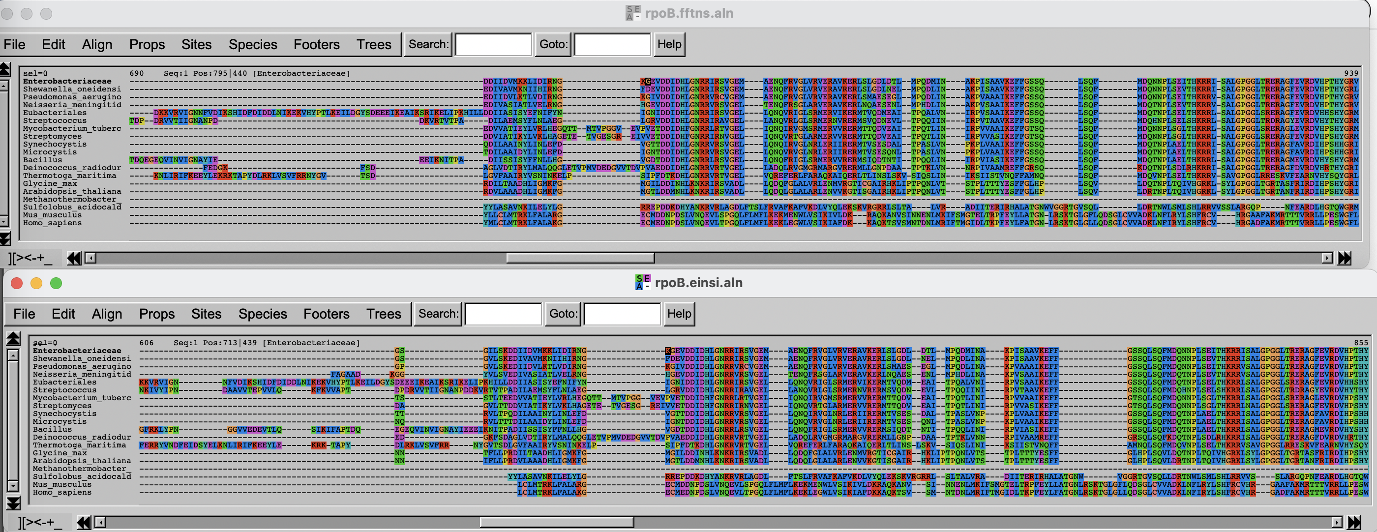
Alignment visualization
You will now inspect the two resulting alignment methods. There are
no convenient way to do that from Uppmax, and the easiest solution is to
download the alignments on your computer and to use
either seaview
(you will need to install it on your computer) or an online alignment
viewer like AlignmentViewer.
Arrange the two windows on top of each other. Change the fontsize (Props -> Fontsize in Seaview) to 8 to see a larger portion of the alignment.
Challenge
Can you spot differences? Which alignment is longer?
Hint: try to scroll to position 800-900. What do you see there? How are the blocks arranged?
If you have time over, spend it exploring the different options of Seaview/AlignmentViewer.
Task 2: Trim the alignment
Often, some regions of the alignment don’t align properly, either because they contain low complexity segments (hinges in proteins) or evolved through repeated insertions/deletions, which alignment program cannot handle properly. It is thus good practice to remove (trim) these regions, as they are likely to worsen the quality of the subsequent phylogenetic trees. On the other hand, trimming too much of the alignment removes also potentially valuable information. There is thus a balance to be found.
In this part, you will use two different alignment trimmers, TrimAl and ClipKIT, on the
results of mafft’s E-INS-i algorithm.
Trimming with TrimAl
First, load the module and look at the list of options available with
trimAl.
trimAl offers a lot of different options. You are going
to explore two different: gap threshold (-gt) and the
heuristic method -automated1, which automatically decides
between three automated methods, -gappyout,
-strict and -strictplus, based on the
properties of the alignment. The gap threshold methods removes columns
that contain a fraction of sequences lower than the cut-off.
For comparison purposes, you will be adding an html output.
Challenge 2.1: TrimAl with gap threshold
Use trimAl to remove positions in the alignment that
have more than 40% gaps.
The “gap threshold” is actually expressed as fraction of non-gap residues.
Challenge 2.2: TrimAl with automated trimming
Use trimAl with the automated heuristic algorithm.
Add a -automated1 option and rerun as above, choosing a
different output file.
Challenge 2.3: Compare the results
Get the files (both alignments and html files) to your own laptop and
visualize the results, by opening the html files with your
browser and the alignment files with seaview or the viewer
you used above.
On your own laptop, go inside the folder where you want to import the
files. Use scp. On some OS it is necessary to escape the
wildcard *. If the output says something about
no matches found, try that.
As before, if you do not have access to a terminal on your windows laptop, use MobaXterm and Session > SFTP to copy files to your computer.
Trimming with ClipKIT
ClipKIT is
one of the more recent tools to trim multiple sequence alignments. In a
nutshell, it tries to preseve phylogenetically-informative sites, rather
than trimming gappy regions. Although it also has multiple options and
modes, you will only use the default mode, smart-gap.
OUTPUT
---------------------
| Output Statistics |
---------------------
Original length: 2043
Number of sites kept: 1543
Number of sites trimmed: 500
Percentage of alignment trimmed: 24.474%

Execution time: 0.379s
Comparing all the results
Import the data and inspect the three alignments.
Challenge 2.5: Import data and compare results
Copy the alignment file and visualize with seaview or
the web-based visualization tool.
Use scp as above.
Then use seaview or another viewer to visualize and
compare results.
The three alignments on top of each other look like this. Click on this link to better see the figure.
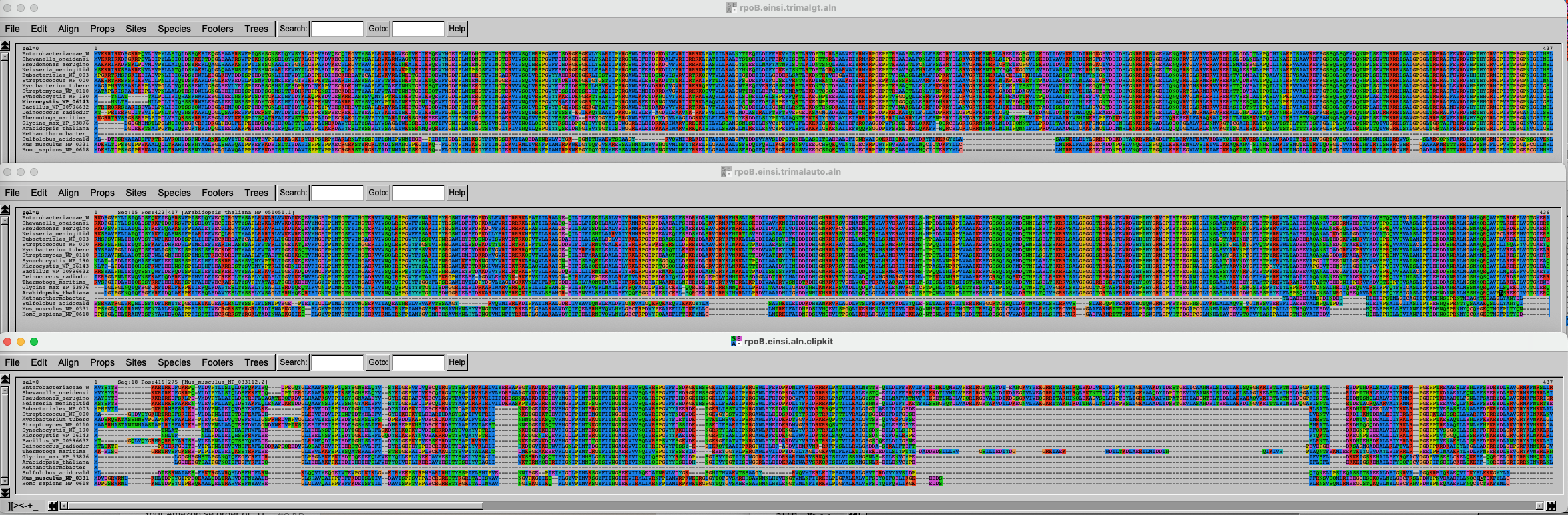
It is of course difficult to draw conclusions based on this figure, but can you spot some trends? What alignment is more likely to generate good results?
Part 2: Phylogenetics
Overview
Questions
- How do you build a simple, distance-based phylogenetic tree?
- How do you build a phylogenetic tree with more advanced methods?
- How do you ascertain statistical support for phylogenetic trees?
Objectives
- Use
mafftto align multiple sequences. - Test different algorithms.
Overview
Questions
- How do you build a simple, distance-based phylogenetic tree?
- How do you build a phylogenetic tree with more advanced methods?
- How do you ascertain statistical support for phylogenetic trees?
Objectives
- Learn the basic of phylogenetics tree building, taking the simplest of the examples with a UPGMA tree.
- Learn how to use phylogenetics algorithms, neighbor-joining and maximum-likelihood.
- Learn how to perform and show bootstraps.
Task 3: Paper-and-pen phylogenetic tree
Setup
The exercise is done for a large part with pen and paper, and then a
demonstration in R on your laptop, using RStudio. We’ll also use the R
package ape, which
you should install if it’s not present on your setup. Commands can be
typed or pasted in the “Console” part of RStudio.
R
install.packages('ape')
OUTPUT
- Querying repositories for available source packages ... Done!
The following package(s) will be installed:
- ape [5.8-1]
These packages will be installed into "~/work/course-microbial-genomics/course-microbial-genomics/renv/profiles/lesson-requirements/renv/library/linux-ubuntu-jammy/R-4.5/x86_64-pc-linux-gnu".

# Installing packages --------------------------------------------------------
[32m✔[0m ape 5.8-1                                [linked from cache]
Successfully installed 1 package in 3.2 milliseconds.
And to load it:
R
library(ape)
UPGMA-based tree
Load the tree in fasta format, reading from a temp
file
R
FASTAfile <- tempfile("aln", fileext = ".fasta")
cat(">A", "----ATCCGCTGATCGGCTG----",
    ">B", "GCTGATCCGTTGATCGG-------",
    ">C", "----ATCTGCTCATCGGCT-----",
    ">D", "----ATTCGCTGAACTGCTGGCTG",
    file = FASTAfile, sep = "\n")
aln <- read.dna(FASTAfile, format = "fasta")
Now look at the alignment. Notice there are gaps, which we don’t want in this example. We also remove the non-informative (identical) columns.
R
alview(aln)
OUTPUT
  000000000111111111122222
  123456789012345678901234
A ----ATCCGCTGATCGGCTG----
B GCTG.....T.......---....
C .......T...C.......-....
D ......T......A.T....GCTG
R
aln_filtered <- aln[,c(7,8,10,12,14,16)]
alview(aln_filtered)
OUTPUT
  123456
A CCCGTG
B ..T...
C .T.C..
D T...AT
Now we have a simple alignment as in the lecture. Dots
(.) mean that the sequence is identical to the top row,
which makes it easier to calculate distances.
Calculating distance “by hand”
Let’s use a matrix to calculate distances between sequences. We’ll just count the number of differences between the sequences. We’ll then group the two closest sequences. Which are they?
| A | B | C | D | |
|---|---|---|---|---|
| A | ||||
| B | ||||
| C | ||||
| D |
Here is the solution:
| A | B | C | D | |
|---|---|---|---|---|
| A | ||||
| B | 1 | |||
| C | 2 | 3 | ||
| D | 3 | 4 | 5 |
The two closest sequences are A and B.
Calculating distance “by hand” (continued)
Let’s now cluster together A and B, and calculate the average distance from AB to the other sequences, weighted by the size of the clusters.
| AB | C | D | |
|---|---|---|---|
| AB | |||
| C | |||
| D |
The average distance for AB to C is calculated as follow:
\(d(AB,C) = \dfrac{d(A,C) + d(B,C)}{2} = \dfrac{2 + 3}{2} = 2.5\)
And so on for the other distances:
| AB | C | D | |
|---|---|---|---|
| AB | |||
| C | 2.5 | ||
| D | 3.5 | 5 |
Calculating distance “by hand” (continued)
Now the shortest distance is AB to C. Let’s recalculate the distance to D again.
| ABC | D | |
|---|---|---|
| ABC | ||
| D |
\(d(ABC,D) = \dfrac{d(AB,D) * 2 + d(C,D) * 1}{2 + 1} = \dfrac{3.5 * 2 + 5 * 1}{3} = 4\)
| ABC | D | |
|---|---|---|
| ABC | ||
| D | 4 |
The tree is reconstructed by dividing the distances equally between the two leaves. - A-B: each 0.5. - AB-C: each side gets 2.5/2 = 1.25. The branch to AB is 1.25 - 0.5 = 0.75 - ABC-D: each side gets 4/2 = 2. The branch to ABC is 2 - 0.75 - 0.5 = 0.75
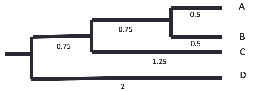
Let’s know do the same using bioinformatics tools.
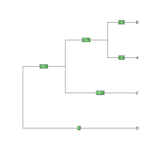
Challenge
We’ll use dist.dna to calculate the distances. We’ll use
a “N” model, that just counts the differences and doesn’t correct or
normalizes. We’ll use the function hclust to perform the
UPGMA method calculation. The tree is then plotted, and the branch
lengths plotted with edgelabels:
R
dist_matrix <- dist.dna(aln_filtered, model="N")
dist_matrix
OUTPUT
  A B C
B 1
C 2 3
D 3 4 5
R
tree <- as.phylo(hclust(dist_matrix, "average"))
plot(tree)
edgelabels(tree$edge.length)
Task 4: Neighbor-joining and Maximum-likelihood tree
Introduction
In the previous episode, we inferred a simple phylogenetic tree using UPGMA, without correcting the distance matrix for multiple substitutions. UPGMA has many shortcomings, and gets worse as distance increases. Here we’ll test Neighbor-Joining, which is also a distance-based, and a maximum-likelihood based approach with IQ-TREE.
Neighbor-joining
The principle of Neighbor-joining method (NJ) is to start from a star-like tree, find the two branches that, if joined, minimize the total tree length, join then, and repeat with the joined branches and the rest of the branches.
Challenge
To perform NJ on our sequences, we’ll use the function inbuilt in
Seaview. First (re-)open the alignment we obtained from
mafft with the E-INS-i method, trimmed with ClipKIT. If it
is not on your computer anymore, transfer it again from Uppmax using
scp or SFTP.
If Seaview is not installed on your computer, download it and install it on your computer.
Challenge (continued)
In the Seaview window, select Trees -> Distance methods. Keep the BioNJ option ticked. BioNJ is an updated version of NJ, more accurate for longer distances. Tick the “Bootstrap” option and leave it at 100. We’ll discuss these later. Then click on “Go”.
What do you see? Is the tree rooted? Is the pattern species coherent with what you know of the tree of life? Any weird results?
Challenge
Redo the BioNJ tree for the other alignment we inferred.
Do you see any differences between the two trees? What can you make out of it?
Maximum likelihood
We will now use IQ-TREE to infer a maximum-likelihood (ML) tree of
the RpoB dataset we aligned with mafft previously. While
you performed the first trees on your laptop, you will infer the ML tree
on Uppmax. As usual, use the interactive command to gain
access to compute time. Go to the phylogenetics folder
created in the MSA episode, and load the right modules.
Challenge
Get to the right folder, require compute time and load the right
modules. The project is uppmax2026-1-93. The module
containing IQ tree is called IQ-TREE.
Then run your first tree, on the ClipKIT-trimmed
alignment.
Here, we tell IQ-TREE to use the alignment
-s rpoB.einsi.clipkit.aln, and to test among the standard
substitution models which one fits best (-m MFP). We also
tell IQ-TREE to perform 1000 ultra-fast bootstraps
(-B 1000). We’ll discuss these later.
IQ-TREE is a very complete program that can do a large variety of phylogenetic analysis. To get a flavor of what it’s capable of, look at its extensive documentation.
Have a look at the output files:
OUTPUT
rpoB.einsi.clipkit.aln.bionj    rpoB.einsi.clipkit.aln.iqtree  rpoB.einsi.clipkit.aln.model.gz
rpoB.einsi.clipkit.aln.ckp.gz   rpoB.einsi.clipkit.aln.log     rpoB.einsi.clipkit.aln.splits.nex
rpoB.einsi.clipkit.aln.contree	rpoB.einsi.clipkit.aln.mldist  rpoB.einsi.clipkit.aln.treefile
There are two important files:
* *.iqtree file provides a text summary of the analysis. *
*.treefile is the resulting tree in Newick
format.
To visualize the tree, open the Beta version of phylo.io.
Click on “add a tree” and copy/paste the content of the
treefile (use e.g. less or cat to
display it) in the box. Make sure the “Newick format” is selected and
click on “Done”.
The tree appears as unrooted. It is good practice to start by ordering the nodes and root it. There is no good way to automatically order the branches in phylo.io as of yet, but rerooting can be done by clicking on a branch and selecting “Reroot”. Reroot the tree between archaea and bacteria. Now the tree makes a bit more sense.
Scrutinize the tree. Is it different from the BioNJ tree generated in Seaview? How?
Challenge
Redo a ML tree from the other alignment (FFT-NS) we inferred with
mafft and display the resulting tree in FigTree.
BASH
iqtree -s <alignment file> <option and text for testing model> <option and test for 1000 fast bootstraps> Import the tree on your computer and load it with FigTree or with phylo.io
Bootstraps
We have inferred four trees:
- Two based on the alignment generated from the E-INS-i algorithm (trimmed by ClipKIT), two from the FFT-NS.
- Two inferred with the BioNJ algorithm and two with the ML algorithm (IQ-Tree)
Along the way, we’ve generated bootstraps for all our trees. Now show them on all four trees.
- For the Seaview trees, tick the ‘Br support’ box
- For the trees shown in phylo.io, click on “Settings” > “Branch & Labels” and above the branch, click the drop-down menu and select “Data”.
Challenge
Compare all four trees. Do you find any significant differences?
What are Glycine and Arabidopsis? What about Synechocystis and Microcystis?
Search for the accession number of the Glycine RpoB sequence on NCBI. Any hint there?
The two plant RpoB sequences are from chloroplastic genomes, and thus branch together with the cyanobacterial sequences, in some of the phylogenies at least.
Challenge (continued)
What about the support values for grouping these two groups? How high are they?
- The simplest of the trees are distance-based.
- UPGMA works by clustering the two closest leaves and recalculating the distance matrix.
- Neighbor-joining is distance-based and fast, but not necessarily very accurate
- Maximum-likelihood is slower, but more accurate
Part 3: Genetic drift
As a practical way to understand genetic drift, let’s play with population size, selection coefficients, number of generations, etc.
Overview
Questions
- How does random genetic drift influence fixation of alleles?
- What is the influence of population size?
Objectives
- Learn the basic of phylogenetics tree building, taking the simplest of the examples with a UPGMA tree.
- Learn how to use phylogenetics algorithms, neighbor-joining and maximum-likelihood.
- Learn how to perform and show bootstraps.
Overview
Questions
- How does random genetic drift influence fixation of alleles?
- What is the influence of population size?
Objectives
- Understand how population size influences the probability of fixation of an allele.
- Understand how slightly deleterious mutations may get fixed in small populations.
Introduction
This exercise is to illustrate the concepts of selection, population size and genetic drift, using simulations. We will use mostly Red Lynx by Reed A. Cartwright.
Another option is to use a web interface to the R learnPopGen package, but the last one is mostly for biallelic genes (and thus not that relevant for bacteria).
Open now the Red Lynx website and get familiar with the different options.
You won’t need the right panel (but feel free to explore). The dominance option in the left panel won’t be used either.
Task 6: Genetic Drift without selection
In the first part, you will only play with the number of generations, the initial frequency and the population size.
- Lower the number of generations to 200.
- Adjust the population size to 1000.
- Make sure the intial frequency is set to 50%.
- Run a few simulations (ca 20).
Did any allele got fixed? What is the range of frequencies after 200 generations?
In my simulations, no allele got fixed, the final allele frequencies range 20-80%
Task 6: Genetic Drift without selection (continued)
Now increase the population to 100’000, clear the graph, and repeat the simulations. What’s the range of final frequencies now?
In my simulations, no allele got fixed, and the final allele frequencies range 45-55%
Task 6: Genetic Drift without selection (continued)
Now decrease the population to 10 individuals, clear the graph and repeat these simulations. What’s the range of final frequencies now?
In my simulations, one allele got fixed quickly, the latest one was at generation 100.
Task 6: Genetic Drift without selection (continued)
What do you conclude here?
It is clear that stochastic (random) variation in allele frequencies strongly affects the probability of fixation of alleles in small populations, not so much in large ones.
Task 7: Genetic Drift with selection
So far we’ve only looked at how allele frequencies vary in the absence of selection, that is when the two alleles provide an equal fitness. What’s the influence of random genetic drift when alleles are not neutral?
The selection strength is equivalent to the selection coefficient, i.e. how much higher relative fitness the new allele provides. A selection coefficient of 0.01 means that the organism harboring the new allele has a 1% increased fitness.
- Increase the number of generations to 1000.
- Set the selection strength to 0.01 (1%).
- Set the population size first to 100’000, then to 1000, then to 100.
How long does it take for the allele to get fixed - in average - with the three population sizes?
About the same time, but the trajectories are much smoother with larger populations. In the small population, it happens that the beneficial allele disappears from the population (although not often).
Task 8: Fixation of slightly deleterious alleles in very small populations
We’re now simulating what would happen in a very small population (or a population that undergoes very narrow bottlenecks), when a gene mutates. We’ll have a very small population (10 individuals), a selection value of -0.01 (the mutated allele provides a 1% lower fitness), and a 10% initial frequency, which corresponds to one individual getting a mutation:
- Set the population to 10 individuals.
- Set generations to 200.
- Set initial frequency to 10%.
- Set the selection strength to -0.01.
Run many simulations. What happens?
Most new alleles go extinct quickly. In my simulations, I usually get one of the slightly deleterious mutations fixed after 20 simulations.
That’s it for that part, but feel free to continue playing with the different settings later.
- Random genetic drift has a large influence on the probability of fixation of alleles in small populations, even for non-neutral alleles.
- Random genetic drift has very little influence of the probability of fixation of alleles in large populations.
- Slightly deleterious mutations can get fixed into the population through random genetic drift, if the population is small enough and the selective value is not too large.
Content from Reads, QC and trimming
Last updated on 2026-04-01 | Edit this page
This episode starts a series of labs where you will trace an outbreak of Mycobacterium tuberculosis, from downloading the reads to making assumptions about the transmissions between patients.
The first part, here, describes how to retrieve all necessary data from public repositories - the raw sequenced data of our isolates and a reference genome. It also introduces for loops which we will use for the rest of our analysis.
Overview
Questions
- Trace an outbreak of Mycobacterium, from reads to phylogenetic tree.
- How can I organize my file system for a new bioinformatics project?
- How and where can data be downloaded?
- How can I describe the quality of my data?
- How can I get rid of sequence data that doesn’t meet my quality standards?
Objectives
- How do you use genomics and phylogenetics to trace a microbial outbreak?
- Create a file system for a bioinformatics project.
- Download files necessary for further analysis.
- Use ‘for’ loops to automate operations on multiple files
- Interpret a FastQC plot summarizing per-base quality across all reads.
- Clean FastQC reads for further analysis.
- Use
forloops to automate operations on multiple files.
Introduction
This part of the course is largely inspired from another tutorial developed by Anita Schürch. We will use (part of) the data described in Bryant et al., 2013.
Background of the data
Epidemiological contact tracing through interviewing of patients can identify potential chains of patients that transmitted an infectious disease to each other. Contact tracing was performed following the stone-in-the-pond principle, which interviews and tests potential contacts in concentric circles around a potential bash case.
Tuberculosis (TB) is an infectious disease caused by Mycobacterium tuberculosis. It mostly affects the lungs. An infection with M. tuberculosis is often asymptomatic (latent infection). Only in about 10% of the cases the latent infection progresses to an active infection during a patients lifetime, which, if untreated, leads to death in about half of the cases. The symptoms of an active TB infection include cough, fever, night sweats, weight loss etc. An active TB infection can spread. Once exposed, people often have latent TB. To identify people with latent TB, a skin test can be applied.
Here we have 7 tuberculosis patients with active TB, that form three separate clusters of potential transmission as determined by epidemiological interviews. Patients were asked if they have been in direct contact with each other, or if they visited the same localities. From all patients, a bacterial isolate was grown, DNA isolated, and whole-genome sequenced on an Illumina sequencer.
The three clusters consist of:
- Cluster 1
- Patient A1 (2011) - sample ERR029207
- Patient A2 (2011) - sample ERR029206
- Patient A3 (2008) - sample ERR026478
- Cluster 2
- Patient B1 (2001) - sample ERR026474
- Patient B2 (2012) - sample ERR026473
- Cluster 3
- Patient C1 (2011) - sample ERR026481
- Patient C2 (2016) - sample ERR026482
The second goal of this lab is to affirm or dispute the inferred transmissions by comparing the bacterial genomes with each other. We will do that by identifying SNPs between the genomes.
Getting your project started
Project organization is one of the most important parts of a sequencing project, and yet is often overlooked amidst the excitement of getting a first look at new data. Of course, while it’s best to get yourself organized before you even begin your analyses,it’s never too late to start, either.
Genomics projects can quickly accumulate hundreds of files across tens of folders. Every computational analysis you perform over the course of your project is going to create many files, which can especially become a problem when you’ll inevitably want to run some of those analyses again. For instance, you might have made significant headway into your project, but then have to remember the PCR conditions you used to create your sequencing library months prior.
Other questions might arise along the way:
- What were your best alignment results?
- Which folder were they in: Analysis1, AnalysisRedone, or AnalysisRedone2?
- Which quality cutoff did you use?
- What version of a given program did you implement your analysis in?
In this exercise we will setup a file system for the project we will be working on during this workshop.
Challenge
We will start by creating a sub directory that we can use for the
rest of the labs. First navigate to your own directory on Uppmax and
start an interactive session. Then confirm that you are in
the correct directory using the pwd command.
You should see the output:
OUTPUT
/proj/g2020004/nobackup/3MK013/<username>Exercise
Use the mkdir command to make the following
directories:
molepi
molepi/docs
molepi/data
molepi/resultsUse ls -R to verify that you have created these
directories. The -R option for ls stands for
recursive. This option causes ls to return the contents of
each subdirectory within the directory iteratively.
You should see the following output:
OUTPUT
molepi/:
data  docs  results

molepi/data:

molepi/docs:

molepi/results:
Selection of a reference genome
Reference sequences (including many pathogen genomes) are available at NCBI’s refseq database
A reference genome is a genome that was previously sequenced and is closely related to the isolates we would like to analyse. The selection of a closely related reference genome is not trivial and will warrant an analysis in itself. However, for simplicity, here we will work with the M. tuberculosis reference genome H37Rv.
Download reference genomes from NCBI
Download the M.tuberculosis reference genome from the NCBI ftp site.
First, we switch to the data subfolder to store all our
data
Download reference genomes from NCBI (continued)
The reference genome will be downloaded programmatically from NCBI
with wget. wget is a computer program that
retrieves content from web servers. Its name derives from World Wide Web
and get.
Find the location of the gzipped fna file for that
reference genome via NCBI’s genome, by finding the FTP site and copying
the link to the *_genomic.fna.gz file and using that as an
argument to wget.
Search for Mycobacterium tuberculosis on the Datasets/Genome
website. Identify the “reference genome” (at the top), click on the
accession number, and find the FTP tab. There is many
files, among which
GCF_000195955.2_ASM19595v2_genomic.fna.gz. Right-click and
copy the link.
Download reference genomes from NCBI (continued)
This file is compressed as indicated by the extension of
.gz. It means that this file has been compressed using the
gzip command.
Extract the file by typing
Make sure that is was extracted
OUTPUT
GCF_000195955.2_ASM19595v2_genomic.fnaThe genome has 4’411’532 bp. The stat command of
seqkit is helpful.
OUTPUT
file                                    format  type  num_seqs    sum_len    min_len    avg_len    max_len
GCF_000195955.2_ASM19595v2_genomic.fna  FASTA   DNA          1  4,411,532  4,411,532  4,411,532  4,411,532
Loops
Loops are key to productivity improvements through automation as they allow us to execute commands repeatedly. Similar to wildcards and tab completion, using loops also reduces the amount of typing (and typing mistakes). Our next task is to download our data (see the introduction to this episode) from the short read archive (SRA) at the European Nucleotide Archive (ENA). There are many repositories for public data. Some model organisms or fields have specific databases, and there are ones for particular types of data. Two of the most comprehensive are the National Center for Biotechnology Information (NCBI) and European Nucleotide Archive (EMBL-EBI). In this lesson we’re working with the ENA, but the general process is the same for any database.
We can do this one by one but given that each download takes about one to two hours, this could keep us up all night. Instead of downloading one by one we can apply a loop. Let’s see what that looks like and then we’ll discuss what we’re doing with each line of our loop.
BASH
for sample in ERR029207 ERR029206 ERR026478 ERR026474 ERR026473 ERR026481 ERR026482
do
  echo -e "$sample"
  wget --spider ftp://ftp.sra.ebi.ac.uk/vol1/fastq/"${sample:0:6}"/"${sample}"/"${sample}"_*.fastq.gz
done
When the shell sees the keyword for, it knows to repeat
a command (or group of commands) once for each item in a list. Each time
the loop runs (called an iteration), an item in the list is assigned in
sequence to the variable, and the commands inside the
loop are executed, before moving on to the next item in the list.
Inside the loop, we call for the variable’s value by putting
$ in front of it. The $ tells the shell
interpreter to treat the variable as a variable name
and substitute its value in its place, rather than treat it as text or
an external command.
In this example, the list is seven accession numbers of reads
belonging to the genomes we are interested in. Each time the loop
iterates, it will assign a sample name to the variable
sample and echo (print) the value of the
variable. In the second line, it will run the wget
command.
The first time through the loop, $sample is
ERR029207. The FTP site at EBI is constructed so that fastq
files are stored in a vol1/fastq subfolder. Read files are
not directly in that subfolder, but grouped in subfolders starting with
the six first characters of the accession number (ERR029 in
the first case), then in the accession number subfolder. To get to the
right place, the file path is constructed with the root path
(ftp://ftp.sra.ebi.ac.uk/vol1/fastq/), to which the first 6
characters of the accession number is added through that special
variable operation ("${sample:0:6}") to get to the right
subfolder. Finally, the correct accession subfolder
("${sample}"), the file name prefix
("${sample}"_*.fastq.gz") and the suffix
(_*.fastq.gz) are added. The * ensures that we
get reads from both ends.
Use {} to wrap the variable so that
.fastq.gz will not be interpreted as part of the variable
name. In addition, quoting the shell variables is a good practice AND
necessary if your variables have spaces in them.
For the second iteration, $sample becomes
ERR029206.
We added a --spider option to wget just for
this exercise, to retrieve only the names of the files and not the
actual file, to spare some time downloading files. The data is present
in the data/fastq subfolder of our group folder:
OUTPUT
ERR026473_1.fastq.gz  ERR026474_2.fastq.gz  ERR026481_1.fastq.gz  ERR026482_2.fastq.gz	ERR029207_1.fastq.gz
ERR026473_2.fastq.gz  ERR026478_1.fastq.gz  ERR026481_2.fastq.gz  ERR029206_1.fastq.gz	ERR029207_2.fastq.gz
ERR026474_1.fastq.gz  ERR026478_2.fastq.gz  ERR026482_1.fastq.gz  ERR029206_2.fastq.gz
For more, check Bash Pitfalls
Follow the Prompt
The shell prompt changes from $ to > and
back again as we were typing in our loop. The second prompt,
>, is different to remind us that we haven’t finished
typing a complete command yet. A semicolon, ;, can be used
to separate two commands written on a single line.
Same Symbols, Different Meanings
Here we see > being used a shell prompt, whereas
> is also used to redirect output. Similarly,
$ is used as a shell prompt, but, as we saw earlier, it is
also used to ask the shell to get the value of a variable.
If the shell prints > or $ then
it expects you to type something, and the symbol is a prompt.
If you type > or $ yourself, it
is an instruction from you that the shell to redirect output or get the
value of a variable.
We have called the variable in this loop sample in order
to make its purpose clearer to human readers. The shell itself doesn’t
care what the variable is called; if we wrote this loop as:
or:
it would work exactly the same way. Don’t do this. Programs
are only useful if people can understand them, so meaningless names
(like x) or misleading names (like pizza)
increase the odds that the program won’t do what its readers think it
does.
Multipart commands
The for loop is interpreted as a multipart command. If
you press the up arrow on your keyboard to recall the command, it may be
shown like so (depends on your bash version):
When you check your history later, it will help your remember what you did!
Link the read files
Now link the files from the data folder, to perform
quality control.
Challenge
All the read files start with ERR and have a fastq.gz
extension. It means they are in fastq format and compressed. Softlink
the files in your molepi/data folder, using a nested loop.
The data/fastq folder is three levels up. For each
accession number there are two fastq.gz files, one for each
end (1 or 2).
Softlinks are done with ln -s. Use the same loop
backbone as above, and nest a for loop over the two ends of
the reads (1 and 2).
Bioinformatics workflows
When working with high-throughput sequencing data, the raw reads you get off of the sequencer will need to pass through a number of different tools in order to generate your final desired output. The execution of this set of tools in a specified order is commonly referred to as a workflow or a pipeline.
An example of the workflow we will be using is provided below with a brief description of each step.
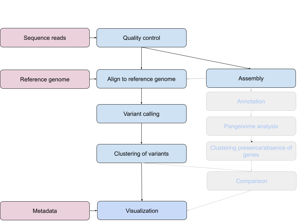
- Quality control - Assessing quality using FastQC
- Quality control - Trimming and/or filtering reads (if necessary)
- Align reads to reference genome - Snippy
- Variant calling - Snippy
- Clustering variants - iTOL
- Assembly - SKESA
- Annotation (extra material)
- Pangenome analysis (extra material)
- Clustering presence and absence of genes (extra material)
- Comparison of clustering methods (extra material)
- Data visualization - Microreact
These workflows in bioinformatics adopt a plug-and-play approach in that the output of one tool can be easily used as input to another tool without any extensive configuration. Having standards for data formats is what makes this feasible. Standards ensure that data is stored in a way that is generally accepted and agreed upon within the community. The tools that are used to analyze data at different stages of the workflow are therefore built under the assumption that the data will be provided in a specific format.
Quality Control
The first step in the variant calling workflow is to take the FASTQ files received from the sequencing facility and assess the quality of the sequence reads.
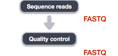
You’ve already seen that part, but repetition doesn’t hurt. If you feel that it’s anyway unnecessary, move on to the next part.
Details on the FASTQ format
Although it looks complicated (and it is), it’s easy to understand the fastq format with a little decoding. Some rules about the format include…
| Line | Description |
|---|---|
| 1 | Always begins with ‘@’ and then information about the read |
| 2 | The actual DNA sequence |
| 3 | Always begins with a ‘+’ and sometimes the same info in line 1 |
| 4 | Has a string of characters which represent the quality scores; must have same number of characters as line 2 |
We can view the first complete read in one of the files our dataset
by using head to look at the first four lines.
Challenge
You will use zcat to extract text from a gzipped file.
OUTPUT
@ERR029206.1 IL31_5505:8:1:6233:1087#4/1
TCNAGTCAGCACACACATGCGAAAGAATCCACCGACTAGGGTCAGCGGGGTTTGCAGTTGGTCGCGGACGTAACCG
+
<='=ABBBBCBBBBBBBBC>BBCBBBBBB@BBBBBB=BCBB@@B@@BB@@,@@@@@@@@@@@@@@@@@@@@@@@@@One of the nucleotides in this read is unknown (N).
Line 4 shows the quality for each nucleotide in the read. Quality is interpreted as the probability of an incorrect base call (e.g. 1 in 10) or, equivalently, the base call accuracy (eg 90%). To make it possible to line up each individual nucleotide with its quality score, the numerical score is converted into a code where each individual character represents the numerical quality score for an individual nucleotide. For example, in the line above, the quality score line is:
OUTPUT
<='=ABBBBCBBBBBBBBC>BBCBBBBBB@BBBBBB=BCBB@@B@@BB@@,@@@@@@@@@@@@@@@@@@@@@@@@@The < character and each of the =
characters represent the encoded quality for an individual nucleotide.
The numerical value assigned to each of these characters depends on the
sequencing platform that generated the reads. The sequencing machine
used to generate our data uses the standard Sanger quality PHRED score
encoding, using by Illumina version 1.8 onwards. Each character is
assigned a quality score between 0 and 40 as shown in the chart
below.
OUTPUT
Quality encoding: !"#$%&'()*+,-./0123456789:;<=>?@ABCDEFGHI
                  |         |         |         |         |
Quality score:    0........10........20........30........40
Each quality score represents the probability that the corresponding nucleotide call is incorrect. This quality score is logarithmically based, so a quality score of 10 reflects a base call accuracy of 90%, but a quality score of 20 reflects a base call accuracy of 99%. These probability values are the results from the base calling algorithm and dependent on how much signal was captured for the base incorporation.
Looking back at our read:
OUTPUT
@ERR029206.1 IL31_5505:8:1:6233:1087#4/1
TCNAGTCAGCACACACATGCGAAAGAATCCACCGACTAGGGTCAGCGGGGTTTGCAGTTGGTCGCGGACGTAACCG
+
<='=ABBBBCBBBBBBBBC>BBCBBBBBB@BBBBBB=BCBB@@B@@BB@@,@@@@@@@@@@@@@@@@@@@@@@@@@
We can now see that the quality of an N (')
is 6, which corresponds to a over 25% error probability:
\(10^{-\frac{6}{10}} \cong 0.25\)
Quality Encodings Vary
Although we’ve used a particular quality encoding system to
demonstrate interpretation of read quality, different sequencing
machines use different encoding systems. This means that, depending on
which sequencer you use to generate your data, a # may not
be an indicator of a poor quality base call.
This mainly relates to older Solexa/Illumina data, but it’s essential that you know which sequencing platform was used to generate your data, so that you can tell your quality control program which encoding to use. If you choose the wrong encoding, you run the risk of throwing away good reads or (even worse) not throwing away bad reads!
Assessing Quality using FastQC
In real life, you won’t be assessing the quality of your reads by visually inspecting your FASTQ files. Rather, you’ll be using a software program to assess read quality and filter out poor quality reads. We’ll first use a program called FastQC to visualize the quality of our reads.Later in our workflow, we’ll use another program to filter out poor quality reads.
FastQC has a number of features which can give you a quick impression of any problems your data may have, so you can take these issues into consideration before moving forward with your analyses. Rather than looking at quality scores for each individual read, FastQC looks at quality collectively across all reads within a sample. The image below shows a FastQC-generated plot that indicates a very high quality sample:
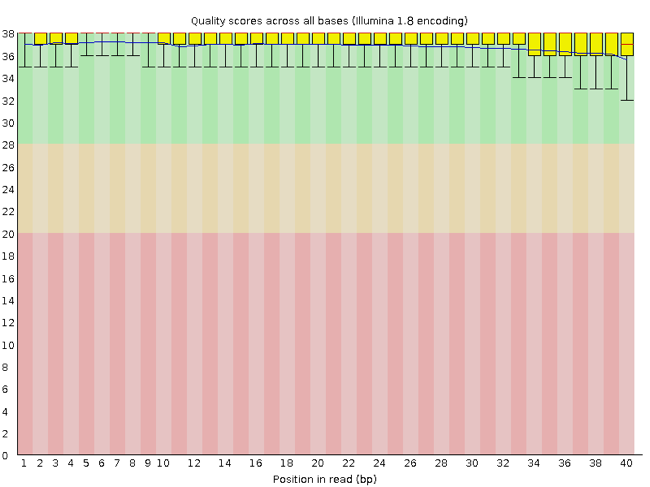
The x-axis displays the base position in the read, and the y-axis shows quality scores. In this example, the sample contains reads that are 40 bp long. For each position, there is a box-and-whisker plot showing the distribution of quality scores for all reads at that position. The horizontal red line indicates the median quality score and the yellow box shows the 2nd to 3rd quartile range. This means that 50% of reads have a quality score that falls within the range of the yellow box at that position. The whiskers show the range to the 1st and 4th quartile.
For each position in this sample, the quality values do not drop much lower than 32. This is a high quality score. The plot background is also color-coded to identify good (green), acceptable (yellow), and bad (red) quality scores.
Now let’s take a look at a quality plot on the other end of the spectrum.
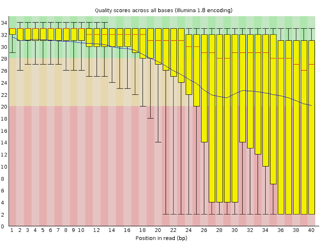
Here, we see positions within the read in which the boxes span a much wider range. Also, quality scores drop quite low into the “bad” range, particularly on the tail end of the reads. The FastQC tool produces several other diagnostic plots to assess sample quality, in addition to the one plotted above.
Running FastQC
Navigate to your FASTQ dataset:
Exercise
We softlinked the samples. How many FASTQ files are in this dataset? Why is this? What is the difference between the two files that start with the same name? Discuss with your neighbour.
There are 14 FASTQ files. Each sample has paired-end reads.
FastQC can accept multiple file names as input, including files that
are compressed (.gz) so we can use the
*.fastq.gz wildcard to run FastQC on both the compressed
FASTQ files for sample ERR029206 in this directory.
You will see an automatically updating output message telling you the progress of the analysis. It will start like this:
OUTPUT
Started analysis of ERR029206_1.fastq.gz
Approx 5% complete for ERR029206_1.fastq.gz
Approx 10% complete for ERR029206_1.fastq.gz
Approx 15% complete for ERR029206_1.fastq.gz
Approx 20% complete for ERR029206_1.fastq.gz
Approx 25% complete for ERR029206_1.fastq.gz
Approx 30% complete for ERR029206_1.fastq.gz
In total, it should take a couple minutes minutes for FastQC to run on our two FASTQ files. When the analysis completes, your prompt will return. So your screen will look something like this:
OUTPUT
Approx 85% complete for ERR029206_2.fastq.gz
Approx 90% complete for ERR029206_2.fastq.gz
Approx 95% complete for ERR029206_2.fastq.gz
Analysis complete for ERR029206_2.fastq.gz
data $
The FastQC program has created several new files within our
/data/ directory.
OUTPUT
...
[...]
ERR029206_1.fastq.gz
ERR029206_1_fastqc.html
ERR029206_1_fastqc.zip
ERR029206_2.fastq.gz
ERR029206_2_fastqc.html
ERR029206_2_fastqc.zip
[...]
For each input gzipped FASTQ file, FastQC has created a
.zip file and a .html file. The
.zip file extension indicates that this is actually a
compressed set of multiple output files. We’ll be working with these
output files soon. The .html file is a stable webpage
displaying the summary report for each of our samples.
We want to keep our data files and our results files separate, so we
will move these output files into a new directory within our
results/ directory.
BASH
mkdir ../results/fastqc_untrimmed_reads
mv *.zip ../results/fastqc_untrimmed_reads/
mv *.html ../results/fastqc_untrimmed_reads/
Now we can navigate into this results directory and do some closer inspection of our output files.
Viewing HTML files
If we are working on our local computers, we may display each of
these HTML files as a webpage. Otherwise, copy the files to your local
computer using scp and use your browser:
You may need to replace the command firefox with the
name of another web navigator if you have one.
Exercise
Discuss your results with a neighbor. Do the sample looks good in terms of per base sequence quality?
Exercise
What are the read lengths of the different samples?
Cleaning Reads
It’s very common to have some reads within a sample, or some positions (near the beginning or end of reads) across all reads that are low quality and should be discarded. We will use a program called seqtk to filter poor quality reads and trim poor quality bases from our samples.
Seqtk Options
Seqtk is a program written in C and aims to be a Swiss Army Knife for sequencing reads. You don’t need to learn C to use Seqtk, but the fact that it’s a C program helps explain the syntax that is used to run Seqtk. Seqtk takes as input files either FASTQ files or gzipped FASTQ files and outputs FASTQ or FASTA files. The basic command to run Seqtk starts like this:
That’s just the basic command, however. Seqtk has a variety of options and parameters. We will need to specify what options we want to use for our analysis. Here are some of the options:
| option | meaning |
|---|---|
seq |
common transformation of FASTA/Q |
comp |
get the nucleotide composition of FASTA/Q |
trimfq |
trim FASTQ using the Phred algorithm |
In addition to these options, there are a number if trimming options available:
| step | meaning |
|---|---|
-q |
error rate threshold (disabled by -b/-e) [0.05] |
-l |
maximally trim down to INT bp (disabled by -b/-e) [30] |
-b |
trim INT bp from left (non-zero to disable -q/-l) [0] |
-e |
trim INT bp from right (non-zero to disable -q/-l) [0]. |
We will use only a few of these options in our analysis. It is important to understand the steps you are using to clean your data.
A complete command for trimming with seqtk will look something like this:
Trimming
Now we will run seqtk trimfq on our data. To begin, make sure you are
still in your data directory:
We are going to run seqtk on one sample giving it an error rate threshold of 0.01 which indicates the base call accuracy. We request that, after trimming, the chances that a base is called incorrectly are only 1 in 10000.
Notice that we needed to redirect the output to a file. If we don’t do that, the trimmed fastq data will be displayed in the console.
Exercise
Use seqtk fqchk to compare the untrimmed and trimmed reads of ERR029206_1 in terms of number of sequenced bases, percentage of A,G,C,T and N and average quality. What do you notice? Discuss with your neighbor.
OUTPUT
min_len: 76; max_len: 76; avg_len: 76.00; 36 distinct quality values
POS #bases  %A  %C  %G  %T  %N  avgQ    errQ    %low    %high
ALL 315791552 18.0 32.1 32.2 17.7 0.0 30.6 21.4 5.4 94.6OUTPUT
min_len: 30; max_len: 76; avg_len: 69.12; 36 distinct quality values
POS #bases  %A  %C  %G  %T  %N  avgQ    errQ    %low    %high
ALL 287211920   18.2    32.0    31.9    17.8    0.0 31.7    28.8    1.3 98.7
We’ve just successfully trimmed one of our FASTQ files! However,
there is some bad news. seqtk can only operate on one
sample at a time and we have more than one sample. The good news is that
we can use a for loop to iterate through our sample files
quickly! This will take a few minutes.
Challenge
Write a loop which trims all .fastq.gz files and
redirect the output into _trim.fastq files.
Create a new variable, built from the input file name (ending in
.fastq.gz).
infile is the first variable in our loop and takes the
value of each of the FASTQ files in our directory. outfile
is the second variable in our loop and is defined by adding
_trim.fastq to the end of our input file name. Use
{} to wrap the variable so that _trim.fastq
will not be interpreted as part of the variable name. In addition,
quoting the shell variables is a good practice AND necessary if your
variables have spaces in them.
For more, check Bash Pitfalls. There
are no spaces before or after the =.
Go ahead and run the for loop. It should take a few minutes for seqtk to run for each of our fourteen input files. Once it’s done running, take a look at your directory contents.
OUTPUT
...
ERR029206_1.fastq.gz_trim.fastq  ERR029206_2.fastq.gz_trim.fastq
We’ve now completed the trimming and filtering steps of our quality
control process! Before we move on, let’s move our trimmed FASTQ files
to a new subdirectory within our data/ directory.
OUTPUT
...
ERR029206_1.fastq.gz_trim.fastq
ERR029206_2.fastq.gz_trim.fastq
Challenge
Again, use seqtk fqchk to compare the untrimmed and
trimmed reads of both samples. Note the number of bases ‘#bases’ of the
trimmed and untrimmed reads. Calculate the theoretical coverage of the
genomes before and after trimming, assuming that all our genomes do have
the same size as our reference genome (4411532 bases).
Hint: Sum up forward and reverse reads!
OUTPUT
min_len: 30; max_len: 76; avg_len: 69.12; 36 distinct quality values
POS #bases  %A  %C  %G  %T  %N  avgQ    errQ    %low    %high
ALL 287211920 18.2 32.0 31.9 17.8 0.0 31.7 28.8 1.3 98.7OUTPUT
min_len: 30; max_len: 76; avg_len: 63.79; 36 distinct quality values
POS #bases  %A  %C  %G  %T  %N  avgQ    errQ    %low    %high
ALL 265048852   18.1    32.1    32.1    17.7    0.0 31.2    25.7    2.5 97.5
Coverage = #bases (forward + reverse) / genome size In this case:
\(125.18 = \dfrac{(287211920 + 265048852)}{4411532}\)
-
wgetis a computer program to get data from the internet -
forloops let you perform the same set of operations on multiple files with a single command - Sequencing data is large
- In bioinformatic workflows the output of one tool is the input of the other.
- FastQC is used to judge the quality of sequencing reads.
- Data cleaning is an essential step in a genomics pipeline.
- We will work towards confirming or disputing transmission in TB cases
- After this practical training you will have some familiarity with working on the command line
Content from Sequence assembly
Last updated on 2026-04-01 | Edit this page
Sequence assembly means the alignment and merging of reads in order to reconstruct the original sequence. The assembly of a genome from short sequencing reads can take a while. We will therefore run this process for two genomes only.
Overview
Questions
- How can the information in the sequencing reads be reduced?
- What are the different methods for assembly?
Objectives
- Understand differences between assembly methods
- Assemble the short reads
Exercise 1: Sequence assembly with SKESA
The assembler we will run is SKESA. SKESA generates a final
assembly from multiple kmers. A list of kmers is automatically selected
by SKESA using the maximum read length of the input data, and each
individual kmer contributes to the final assembly. If desired, the
lengths of kmers can be specified with the --kmer and
--steps flags which will adjust automatic kmer
selection.
Because assembly of each genome would take a long time, you will only run one assembly here.
Preparation
Start the interactive session, go to the molepi
subfolder, create a results/assembly subfolder. Then go to
the folder containing the fastq files (data/trimmed_fastq)
that you created in the previous tutorial.
Running SKESA in a loop
To run SKESA we will use the skesa command with a number of option that we will explore later on. We can start the loop (again, a short loop with only one sample in this actual case to spare computing resources) with the assemblies with:
BASH
module load SKESA
for sample in ERR029206
do
skesa \
--cores 2 \
--memory 8 \
--fastq "${sample}"_1.fastq.gz_trim.fastq "${sample}"_2.fastq.gz_trim.fastq 1> ../../results/assembly/"${sample}".fasta
done
A non-quoted backslash, \ is used as an escape character
in Bash. It preserves the literal value of the next character that
follows, with the exception of newline. This means that the back slash
starts a new line without starting a new command - we only add it for
better readability.
The output redirection sign (1>) is different than
the ususal >. It specifies that only the standard output
(i.e. generally the results) will go to that file, while the standard
error (i.e. warning and error messages, or other logging information)
are displayed on the console. To save the standard error to a file, use
2>, e.g.
The assembly should take about 5 minutes per genome, using 2 cores and 8 GB of memory.
Downloading the missing assemblies
If you haven’t assembled all samples, download the finished contigs
to your computer and decompress them. They will decompress in a folder
called assembly, so one solution is to rename the assembly
folder you already have to something else:
BASH
cd ../../results/
mv assembly partial_assembly
tar xvzf /proj/g2020004/nobackup/3MK013/data/assemblies.tar.gz
ls assembly
OUTPUT
ERR026473.fasta ERR026478.fasta ERR026482.fasta ERR029207.fasta
ERR026474.fasta ERR026481.fasta ERR029206.fastaChallenge: What do the command line parameters of SKESA mean?
Find out a) the version of SKESA you are using and b) what the used command line parameters mean.
OUTPUT
skesa -h
..
General options:
-h [ --help ]                 Produce help message
-v [ --version ]              Print version
..
--cores arg (=0)              Number of cores to use (default all) [integer]
--memory arg (=32)            Memory available (GB, only for sorted counter)
..
--fastq arg                   Input fastq file(s) (could be used multiple times for different runs) [string]
..
..
Examine the results of the assembly
You will now explore the files output by SKESA. Find out the number of contigs, and the various assembly statistics.
What do the they mean? What are N50, L50, N80 and L80?
Challenge: How many contigs were generated by SKESA?
Find out how many contigs there are in the M. tuberculosis
isolates. Use for example the GenomeTools software, available as
module with the same name on Uppmax. The main program is called
gt. The documentation is comprehensive and can be found on
the website or via the command line. We are looking for some subcommand
that can give use statistics on sequences.
OUTPUT
# number of contigs:     390
# total contigs length:  4239956
# mean contig size:      10871.68
# contig size first quartile: 989
# median contig size:         5080
# contig size third quartile: 15546
# longest contig:             74938
# shortest contig:            200
# contigs > 500 nt:           323 (82.82 %)
# contigs > 1K nt:            291 (74.62 %)
# contigs > 10K nt:           148 (37.95 %)
# contigs > 100K nt:          0 (0.00 %)
# contigs > 1M nt:            0 (0.00 %)
# N50                25167
# L50                54
# N80                11379
# L80 129Challenge: Compare the results of the different samples
How to compare assemblies? What do N50 and L50 mean?
How could you get N50 stats for all the assemblies?
Wikipedia is your friend: https://en.wikipedia.org/wiki/N50,_L50,_and_related_statistics
Write a for loop over accessions, printing the accession
name and running gt on each fasta file. Grepping for the
information you want. You can grep two different patterns by prefixing
each pattern with -e. E.g.
grep -e "this" -e "that" greps this or that.
Exercise 2: assembly with SPAdes
To compare how different assemblers perform, you will also use SPAdes. SPAdes is a very versatile and can assemble many different data types, including combining long and short reads.
Challenge: Assemble the genomes with SPAdes
You will only perform the assembly on one genome, but use the loop
form anyway. You will use the --isolate mode, but the
--careful mode would also be interesting. This might take
5-10 minutes per genome.
SPAdes can be loaded with the SPAdes module, and the
main command is spades.py. Make a
spades_assembly folder in the molepi/results
folder and go there. Then run a 1-genome loop as above. SPAdes has
arguments -1 and -2 for reads from two ends,
the -o to use a specific folder to store the output (use
<accession>_spades), -t to use several
threads (use 2), and -m to set the maximum memory in Gb
(use 8).
BASH
Folders etc:
BASH
cd /proj/g2020004/nobackup/3MK013/<username>/molepi/results
mkdir spades_assembly
cd spades_assembly
Running SPAdes
BASH
module load <module>
for accession in ERR029206
do
  <print the accession with echo>
  spades.py \
    <mode isolate> \
    <flag for read file 1> ../../data/trimmed_fastq/"${accession}"_1.fastq.gz_trim.fastq \
    <flag for read file 2> ../../data/trimmed_fastq/"${accession}"_2.fastq.gz_trim.fastq \
    -o <output folder> \
    <options for 2 threads and 8 Gb memory>
doneChallenge: Compare the results of the assembly with SPAdes and SKESA
Using Genome Tools, compare the result of the two assemblies.
Exercise 3: Preliminary annotation
Physical annotation
The goal here is to find ORFs and start codons, and thus identify proteins in the genome.
Challenge: Use prodigal
Find how prodigal works and use it to annotate the proteome of
ERR029206. Make an annotation folder in the
molepi/results folder. Use default settings, only setting
the input file -i and writing the protein translations
(-a) to a .faa file. Redirect the standard
output (>) to a .gbk file. For both files,
use the accession number as prefix.
Examine the resulting files, both the .faa and the
.gbk. Can you make sense of the information there?
Functional annotation
The physical annotation provided by prodigal identifies genes (ORFs and start codons), but it does not give any information about the function of the genes identified. The next step is thus to infer a function for each of the identified genes. This process usually involves aligning the proteins to different databases, e.g. using BLAST and other programs. You will not perform a full functional annotation in this exercise, but you will try to use blastp to find a RpoB (RNA polymerase B) homolog in the genome.
Create a BLAST database
With the proteome (.faa file) of sample ERR029206,
create a BLAST database, of protein type. Use the
makeblastdb function that comes with the BLAST package.
Find rpoB homologs
Now that you made the database, use the RpoB sequence from E. coli that you retrieved in the BLAST exercise to find whether there are one or several RpoB homologs in the proteome you just annotated. Examine the BLAST results: how many homologs to RpoB in that genome?
- Assembly is a process which aligns and merges fragments from a longer DNA sequence in order to reconstruct the original sequence.
- k-mers are short fragments of DNA of length k
Content from Protein structure prediction
Last updated on 2026-04-01 | Edit this page
Overview
Questions
- How can we predict a protein’s 3D structure from its sequence?
- How do we evaluate the confidence of predicted structures?
Objectives
- Predict protein and protein complex structure using
AlphaFold. - Interpret prediction confidence scores.
- Visualize predicted structures.
- Compare predicted structures to known structures.
Introduction
In this episode, we are going to explore protein structure
prediction. For structure prediction, you are going to use AlphaFold,
a deep learning model based tool developed by DeepMind that has
revolutionized the field of protein structure prediction. We will (1)
predict the structure of a protein, (2) interpret the confidence of the
predictions, (3) visualize the predicted structures, and (4) compare
them to known structures. Let’s get started by setting up our
environment for prediction and loading the necessary libraries.
Task 1: Predicting structure of a protein
We will use the AlphaFold/3.0.1 module from Pelle for
protein structure prediction. Let’s start!
Challenge 1.1: prepare the terrain
First, using your username and password you need to login to Pelle.
The course base folder is at
/proj/g2020004/nobackup/3MK013. Go to your own folder,
create a protein-structure-exercise subfolder, and move
into it.
Challenge 1.2: upload the AlphaFold3 parameters file
Probably you already have downloaded the AlphaFold3 models using this link.
First, we need to create a params sub-directory under
protein-structure-exercise directory to store the
AlphaFold3 parameters file on Pelle. Then we will upload the parameters
file from the local machine into that params directory on
Pelle.
Use mkdir command to create a new directory, and upload
the file into the params directory using scp
command.
BASH
# create params directory on Pelle
mkdir <basefolder>/<username>/protein-structure-exercise/params
# Open a new terminal on your local machine and use the following command to upload the parameters file to Pelle. Remember to replace `<path_to_parameters_file>` and `<username>` accordingly.
scp <path_to_parameters_file> <username>@pelle.uppmax.uu.se:<basefolder>/<username>/protein-structure-exercise/params
Challenge 1.3: prepare the input file
AlphaFold takes the amino acid (AA) sequence of a protein as input and predicts its 3D structure. For this task, we will use the AA sequence of Adenylate kinase from Escherichia coli (UniProt ID: P69441). You can download the sequence of Adenylate kinase using the following code:
This will download the FASTA file containing the amino acid sequence of the protein.
Q.1 Can you tell how many amino acids are in the sequence? You can
use the grep command to count.
The grep -v ">" command removes the header line,
tr -d '\n' removes newlines, and wc -c counts
the number of characters, which corresponds to the number of amino
acids.
Challenge 1.3: prepare the input file (continued)
You can check how AlphaFold3 input files look like here. You can manually format the input file according to the specifications. But for this exercise, we will use a script that automates the process.
First, we create a directory called af3-input:
Use mkdir command to create a new directory.
Challenge 1.3: prepare the input file (continued)
Now use the following command to prepare the input file for AlphaFold3:
This command will take the FASTA file as input and generate a JSON
file that can be used as AlphaFold3 input. You can inspect the structure
of the JSON file using the cat or less
command.
Q.2 Can you explain why the P69441.json file has its version set to 1 ? Does it follow AlphaFold3 input specification?
Check AlphaFold3 input file preparation instruction here
Check the section about versions in the AlphaFold3 input file preparation instruction.
Challenge 1.4: run AlphaFold3 prediction
Now that we have the input file ready, we can run the
AlphaFold3 prediction.
First, we create output directory for storing the AF3 predicted results:
Now, we will load the AlphaFold3 module, which allows us
to run an already installed version AlphaFold3. Use the following
command:
You should check whether the module is actually loaded by using the following command:
We will run AlphaFold3 using slurm. You
can check the instructions. For this course, we will use a script that
generates a ready-to-use slurm command.
Then, we can run the prediction using the following command:
BASH
python3 <basefolder>/scripts/create_af3_slurm_job.py -p <Project-Code> -i ./af3-input/P69441.json -o ./af3-output -m ./params > job.shNow we execute the job as following:
This command runs the AlphaFold3 prediction using the input JSON file
and saves the results in the af3-output directory. You can
check the status of your job using the
squeue -u <username> command.
Q.3 How long did the prediction take?
You can check the log file generated by the slurm
job.
The log file will have a name like
slurm-<job_id>.out.
Task 2: Interpret the confidence score of the predictions
Now that we have generated a predicted structure, we will evaluate how reliable it is.
In the output directory (af3-output), you will find
several files. One with the suffix
_summary_confidences.json, contains the confidence scores
for the predicted structure. You can use the following command to view
the contents of the confidence summary file:
The predicted template modeling (pTM) score and the interface predicted template modeling (ipTM) score are both derived from a measure called the template modeling (TM) score. This measures the accuracy of the entire structure. A pTM score above 0.5 means the overall predicted fold for the complex might be similar to the true structure. ipTM measures the accuracy of the predicted relative positions of the subunits within the complex. Values higher than 0.8 represent confident high-quality predictions, while values below 0.6 suggest likely a failed prediction. ipTM values between 0.6 and 0.8 are a gray zone where predictions could be correct or incorrect. source.
Challenge 2.1: checking prediction quality
Q.4 What are the pTM and ipTM scores for the predicted structure of Adenylate kinase? Does it indicate a good prediction?
You can find the pTM and ipTM scores in the
_summary_confidences.json file. Look for the keys
"pTM" and "ipTM" in the JSON file.
First find the confidence scores using the command below:
A pTM score above 0.5 suggests the overall fold is likely
correct.
High ipTM values (e.g. >0.8) indicate confident prediction of
interactions.
If your scores fall in these ranges, the prediction is likely
reliable.
Task 3: Visualize the predicted structures
To visualize the predicted structure, you can use a molecular visualization tool such as PyMOL. In case you can not install these tools on your local machine, you can use the web-based tool RCSB 3D View to visualize the predicted structure. However, for this course we will use PyMOL and here is the installation instruction link.
To visualize the predicted structure using PyMOL, you can follow these steps:
Download the predicted structure file (with suffix
_model.cif) from the af3-output directory to
your local machine.
You can use the scp command to securely copy the file
from the remote server to your local machine. Replace
<username> with your actual username and
<local_path> with the path where you want to save the
file on your local machine.
BASH
scp <username>@pelle.uppmax.uu.se:<basefolder>/<username>/protein-structure-exercise/af3-output/p69441/p69441_model.cif <local_path>To visualize in PyMOL, first open PyMOL software on your local machine. PyMol has it’s own command line interface, just like the terminal. You can use that terminal and type the following command to load the predicted structure file:
Task 4: Compare predicted structures to known structures
From UniProt Db entry for Adenylate kinase (P69441), we can see that there are several known structures for this protein in the Protein Data Bank (PDB).
You can find the PDB IDs for the known structures in the UniProt
entry under the “Structure” section. For this exercise, we will compare
our predicted structure to the known structure with PDB ID
1AKE.
Using PyMol terminal, you can fetch the known structure from the PDB database using the following command:
You can then align the predicted structure to the known structure using the following command:
This will align the predicted structure (P69441_model) to the known structure (1AKE) and provide you with an RMSD (Root Mean Square Deviation) value, which indicates how closely the predicted structure matches the known structure. A lower RMSD value indicates a better match.
You can also superimpose the two structures to visually compare them using the following command:
This will superimpose the predicted structure onto the known structure, allowing you to visually assess the similarities and differences between the two structures.
Challenge 4.1: checking structural alignment
Q.5 What is the RMSD value between the predicted structure and the known structure? Does it indicate a good prediction?
Align predicted structure with the known structure from PDB database, using PyMOL.
A low RMSD (e.g. <2 Å) indicates strong agreement with the known
structure.
Higher values suggest deviations and lower prediction accuracy.
Task 5: Predict structure of a protein complex
In this section, we will predict structure of a protein complex 4fqb, where one protein is a toxic effector Tse1 and the other one is an immune protein Tsi1. They together form a protein complex, soon we will see their complex structure.
Let’s begin with copying the FASTA file from <basefolder>/<username>/protein-structure-exercise
directory. The file we need to copy is called
4fqb.fasta.
Then, we prepare the AlphaFold3 input JSON file using
the fasta_to_af3_json.py script. Use the following
command:
Next, you need to run AlphaFold3 prediction using
af3-input/4fqb.json file as input. It is very similar as
the steps described in Challenge 1.4. Only exception is when you use
create_af3_slurm_job.py script, the input (-i) should be
changed as -i af3-input/4fqb.json. See below:
Check whether the AlphaFold3 module is still loaded:
If not, load AlphaFold3 module:
Check whether the module is now loaded successfully:
Then, we create slurm job:
BASH
python3 <basefolder>/scripts/create_af3_slurm_job.py -p <Project-Code> -i ./af3-input/4fqb.json -o ./af3-output -m ./params > job_complex.shNow we execute the job as following:
Challenge 2: check the confidence score, visualise and compare the predicted complex with experimentally derived structure
After the prediction is complete, check the confidence score and compare the predicted structure with the known structure from the PDB database (4FQB) using instruction from Task 2, 3 and 4.
Q.6 Based on the confidence score and RMSD value, do you think AlphaFold3 performed well in predicting the protein complex?
If both confidence scores (pTM/ipTM) are high and RMSD is low,
AlphaFold3 performed well.
If scores are low or RMSD is high, the prediction may be unreliable.
In this episode, we explored how to predict, evaluate, and validate protein structures using AlphaFold3.
- AlphaFold predicts structure from sequence
- pTM/ipTM indicate confidence
- RMSD measures structural similarity
Content from Mapping
Last updated on 2026-04-01 | Edit this page
In this episode we will try to pinpoint single nucleotide polymorphism (SNPs), also called single nucleotide variants (SNVs), between our samples and the reference. The SNPs are determined by a process called read mapping in which reads are aligned to the reference sequence.
Overview
Questions
- How to generate a phylogenetic tree from SNP data?
Objectives
- Map reads against a reference genome
- Extract single nucleotide polymorphisms
- Establish a phylogenetic tree from the SNP data
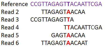
The identified SNPs will be used to compare the isolates to each other and to establish a phylogenetic tree.
SNP calling
snippy is a pipeline that contains different tools to determine SNPs in sequencing reads against a reference genome. It takes forward and reverse reads of paired-end sequences and aligns them against a reference.
Challenge
First we’ll start the interactive session, load the snippy module and
create a snps folder in the molepi/results to
hold the results from snippy.
Snippy is fast but a single run still takes about 15 minutes. We would therefore tell snippy to run all the samples after each other. However this time we cannot use a wildcard to do so. We would instead run all the samples in a loop. The “real” loop is commented out, and we use one that runs only the sample we’ve analyzed so far.
BASH
cd ../data/trimmed_fastq/
#for sample in ERR026473 ERR026474 ERR026478 ERR026481 ERR026482 ERR029206 ERR029207
for sample in ERR029206
do
snippy --ram 8 --outdir ../../results/snps/"${sample}" --ref ../GCF_000195955.2_ASM19595v2_genomic.fna --R1 "${sample}"_1.fastq.gz_trim.fastq --R2 "${sample}"_2.fastq.gz_trim.fastq
done
Here, we provide snippy with an output folder
(--outdir), the location of the reference genome
(--ref), and the trimmed read files for each end of the
pair (--R1 and --R2). We also indicate that
snippy should use 8 Gb of memory (--ram 8).
OUTPUT
CHROM	POS	TYPE	REF	ALT	EVIDENCE	FTYPE	STRAND	NT_POS	AA_POS	EFFECT	LOCUS_TAG	GENE	PRODUCT
NC_000962.3	1849	snp	C	A	A:217 C:0
NC_000962.3	1977	snp	A	G	G:118 A:0
NC_000962.3	4013	snp	T	C	C:176 T:0
NC_000962.3	7362	snp	G	C	C:156 G:0
NC_000962.3	7585	snp	G	C	C:143 G:0
NC_000962.3	9304	snp	G	A	A:127 G:0
NC_000962.3	11820	snp	C	G	G:164 C:0
NC_000962.3	11879	snp	A	G	G:125 A:0
NC_000962.3	14785	snp	T	C	C:163 T:1
This list gives us information on every SNP that was found by snippy when compared to the reference genome. The first SNP is found at the position 1849 of the reference genome, and is a C in the H37Rv (reference strain) and an A in isolate ERR029206. There is a high confidence associated with this SNP: an A has been found 217 times in the sequencing reads and never a C at this position.
Now copy a reduced version of the results obtained from the other
samples, save it in the results folder. We will also rename
the existing snps folder to save it. We extract them from
the archive in the data folder, using tar.
tar is a program to take multiple files, including their
folder structure and put them in a single tar “ball”. Often
the tarballs are compressed with gzip.
BASH
cd /proj/g2020004/nobackup/3MK013/<username>/molepi/results
mv snps snps_partial
mkdir snps
cd snps
tar xvzf ../../../../data/snps.tar.gz
ls *
OUTPUT
ERR026473:
ref.fa.          snps.bam.bai  snps.filt.vcf  snps.log	     snps.tab  snps.vcf.gz
ref.fa.fai	     snps.bed      snps.gff       snps.raw.vcf   snps.txt  snps.vcf.gz.csi
snps.aligned.fa  snps.csv      snps.html      snps.subs.vcf  snps.vcf

ERR026474:
ref.fa		       snps.bam.bai  snps.filt.vcf  snps.log	     snps.tab  snps.vcf.gz
ref.fa.fai	     snps.bed      snps.gff       snps.raw.vcf   snps.txt  snps.vcf.gz.csi
snps.aligned.fa  snps.csv      snps.html      snps.subs.vcf  snps.vcf
Note the unusual way to pass arguments to tar with just
xvzf instead of -x -v -z -f or
-xvzf. x tells tar to extract the archive
(c would be used to create the archive); v is
for verbose, providing more information on the output; z
tells tar to decompress the file; f tells what file to work
on.
The folders don’t contain everything that is output by
snippy, to save space. But it is enough to run
snippy-core, which summarizes several snippy
runs.
Challenge: How many SNPs were identified in each sample??
Find out how many SNPs were identified in the M.
tuberculosis isolates when compared to H37Rv. Hint: The
.txt file in the snippy output contains summary
information:
Challenge: How many SNPs were identified in each sample?? (continued)
OUTPUT
DateTime        2023-05-17T13:51:57
ReadFiles       [...]/data/trimmed_fastq/ERR029207_1.fastq.gz_trim.fastq [...]/data/trimmed_fastq/ERR029207_2.fastq.gz_trim.fastq
Reference       [...]/data/GCF_000195955.2_ASM19595v2_genomic.fna
ReferenceSize   4411532
Software        snippy 4.6.0
Variant-COMPLEX 32
Variant-DEL     57
Variant-INS     52
Variant-MNP     2
Variant-SNP     1290
VariantTotal    1433
This M. tuberculosis isolate contains 1290 SNPs compared to H37Rv.
Repeat this for the other isolates. How about using a
for loop?
Core SNPs
In order to compare the identified SNPs with each other we need to know if a certain position exists in all isolates. A core site can have the same nucleotide in every sample (monomorphic) or some samples can be different (polymorphic).
In this second part, after identifying them, snippy will concatenate the core SNPs, i.e. ignoring sites that are monomorphic in all isolates and in the reference. Concatenation of the SNP sites considerably reduces the size of the alignment.
The --ref argument provides the reference genome. Each
folder containing the result of the previous step of snippy
is then added to the command line.
BASH
cd /proj/g2020004/nobackup/3MK013/<username>/molepi/results/snps
snippy-core --ref=../../data/GCF_000195955.2_ASM19595v2_genomic.fna ERR026473 ERR026474 ERR026478 ERR026481 ERR026482 ERR029206 ERR029207
Instead of writing all samples explicitly, we could use wildcards:
BASH
cd /proj/g2020004/nobackup/3MK013/<username>/molepi/results/snps
snippy-core --ref=../../data/GCF_000195955.2_ASM19595v2_genomic.fna ERR*
The last few lines look like this:
OUTPUT
...
Loaded 1 sequences totalling 4411532 bp.
Will mask 0 regions totalling 0 bp ~ 0.00%
0	ERR026473	snp=1378	del=174	ins=165	het=747	unaligned=125683
1	ERR026474	snp=1369	del=180	ins=143	het=811	unaligned=123020
2	ERR026478	snp=1381	del=221	ins=143	het=638	unaligned=112145
3	ERR026481	snp=1349	del=215	ins=138	het=754	unaligned=126217
4	ERR026482	snp=1348	del=215	ins=145	het=911	unaligned=127554
5	ERR029206	snp=1352	del=152	ins=98	het=1839	unaligned=122677
6	ERR029207	snp=1355	del=152	ins=97	het=1900	unaligned=118570
Opening: core.tab
Opening: core.vcf
Processing contig: NC_000962.3
Generating core.full.aln
Creating TSV file: core.txt
Running: snp-sites -c -o core.aln core.full.aln
This analysis is totally hard-core!
Done.
Our output was written to ‘core.aln’. But let’s have a look at the results.
Discussion: What’s in the output of snippy??
Have a look at the content of these three files>
core.aln
core.full.aln
core.tab
core.txt
What is the difference between these files? Why is
core.aln smaller than core.full.aln? What is
in core.aln?
Phylogenetic tree
We will here infer a phylogenetic tree from the file ‘core.aln’ with IQ-TREE.
In this case, we want IQ-TREE to automatically select the best
(nucleotide) substitution model. IQ-TREE does that by testing many
(among a very large collection) substitution models. We also have SNP
data, which by definition do not contain constant (invariable) sites. We
thus input the alignment with the -s option and the model
with -m MFP+ASC. MFP will tell IQ-TREE to test
a range of models, and ASC will correct for the fact that
there is no constant sites.
Challenge
Infer a phylogenetic tree with IQ-TREE, using the aligned polymorphic
sites identified by snippy-core above. IQ-TREE should find
the best possible model, adding the correction for no constant sites.
Don’t forget to load the right module.
OUTPUT
...
Total wall-clock time used: 0.312 sec (0h:0m:0s)

Analysis results written to:
  IQ-TREE report:                core.aln.iqtree
  Maximum-likelihood tree:       core.aln.treefile
  Likelihood distances:          core.aln.mldist
  Screen log file:               core.aln.log

Date and Time: Thu May 18 09:00:37 2023
With this small data set, IQ-TREE finishes very quickly. Let’s put the resulting files into a separate folder and let’s rename our resulting tree.
Let’s inspect our tree, and give it another extension to make it clear it is a newick file.
OUTPUT
(ERR026473:0.0004854701,ERR026474:0.0004356437,((((ERR026478:0.0000010000,ERR029207:0.0000010000):0.0000010000,ERR029206:0.0000131789):0.0006712219,Reference:0.0075887710):0.0000152316,(ERR026481:0.0000066238,ERR026482:0.0000131899):0.0005602421):0.0002373720);This does not look much like a tree yet. The tree is written in a bracket annotation, the Newick format. In order to make sense of it we can better view this in a tree viewer.
Challenge: Can you identify what substitution model IQ-TREE used?
What model was selected? How does IQ-TREE choose between different models? What does e.g. “JC+ASC+G4” means?
The log file of IQ-TREE contains a lot of information.
The IQ-TREE website contains a description of the DNA substitution models.
OUTPUT
...
Best-fit model according to BIC: TVMe+ASC
...
IQ-TREE chose the TVMe+ASC model. We’ve discussed the ASC above, and you can read more about the TVMe in the IQ-TREE manual. In short, it is a mdoel where base frequencies are deemed equal, and all rates estimated independently, except the rates of transversions (A <-> G and C <-> T) are equal.
The model selection process is also described on the IQ-TREE website.
Challenge: Visualize the tree on your computer
Copy the tree in Newick format (core.aln.newick) to your
computer using scp and use FigTree or phylo.io to visualize it. Do you see a way
to assess the quality of the tree?
Challenge: Rerun the tree, calculating bootstraps this time
In the Phylogenetics module, we
calculated 1000 UltraFast bootstraps using the -B 1000
option. Here, calculate 100 non-parametric bootstraps. Non-parametric
bootstraps are bootstraps that are calculated without making assumptions
about the data. In that case, it means actually resampling the alignment
and calculating trees for each of the bootstrapped alignments. It is a
much slower process than the UltraFast method (which is parametric), but
in that case, since the alignment is very small, the computational load
is acceptable.
With IQ-TREE, non-parametric
bootstraps are inferred using the
-b <n bootstraps> option. Make sure all files are
prefixed with core.aln.100npb (option
--prefix).
The process will take a minute or so. Then in the
results folder, next to the tree folder,
create a tree100npb folder and move the results file
there.
Challenge: Can you identify what substitution model IQ-TREE used? (continued)
When that finishes, copy the resulting tree to your local computer
and visualize it. Display support values: - With FigTree: on the left
menu, tick “Branch labels”, and choose the last row (what you entered
when prompted to do so, label by default) - With phylo.io:
when loading the tree, tick the “Use internal label for branches”. Then
click on “Settings” > “Branches & Labels”, use the drop menu “A”
under “Node labels” and choose “Data”.
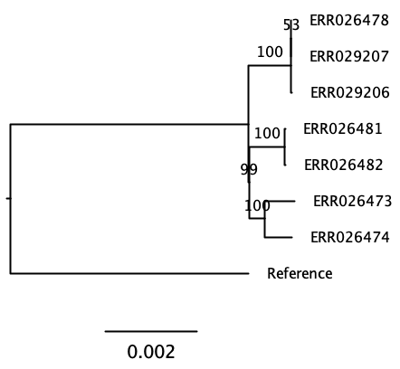
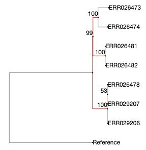
As shown by phylo.io, beta version. Note the position of the “99”.
- Single nucleotide polymorphisms can be identified by mapping reads to a reference genome
- Parameters for the analysis have to be selected based on expected outcomes for this organism
- Concatenation of SNPs helps to reduce analysis volume
- Phylogenetic trees can be written with a bracket syntax in Newick format
Content from Molecular epidemiology
Last updated on 2026-04-01 | Edit this page
The low mutation rate of M. tuberculosis means that even at the highest resolution provided by whole genome sequencing it is still difficult to confidently affirm the inferences of transmission made by traditional epidemiological techniques. This means it is very difficult to determine transmission inclusively. However, whole genome sequencing does in some cases allow us to exclude direct transmission, by using the phylogenetic context provided by other strains. Not only does whole genome sequencing provide the inter-cluster differentiation provided by current typing methods, but it also achieves intra-cluster resolution which can be used to inform epidemiological investigation.
Overview
Questions
- How are phylogenetic trees viewed and compared?
- How can I visualize several layers of data?
- In which cases is transmission likely?
Objectives
- Explore the resulting trees in conjunction with the meta data.
- Make an estimation on the likelihood of transmission events
- Compare and interpret the different data sources.
Comparison of clustering results
We grouped (clustered) our isolates by the information that we extracted from the sequencing reads. We compared our isolates to a reference genome and clustered them on basis of the single nucleotide variations that they exhibit when compared to this reference.
Next, we will visualize this clustering in the context of the meta data. Make sure you have the SNP tree that you generated (or can be downloaded here core.aln.newick) on your own computer. Download also the metadata file.
Visualization of genetic information and metadata
Visualization is frequently used to aid the interpretation of complex datasets. Within microbial genomics, visualizing the relationships between multiple genomes as a tree provides a framework onto which associated data (geographical, temporal, phenotypic and epidemiological) are added to generate hypotheses and to explore the dynamics of the system under investigation.
- Open Chrome. Go to microreact.
- Click on ‘Upload’. Drag-and-drop the newick tree produced by snippy and IQ-TREE (core.aln.newick).
- Click on “Add more files” and select the the metadata file, which is a table comprising metadata file. Choose ‘Data (csv or tsv)’ as file kind.
- Click on continue.
First, the tree should be rooted with the reference strain (the one that has the longest branch). Hover over the middle of the long branch, until a circle appears. Right-click on it, and select “Set as root (re-root)”.
Explore the location, time and further meta data. Play around with the different visualization options with the help of the documentation of microreact.
Discussion
- Which transmission events are likely based on the metadata (location, RFLP, date) alone?
- Which transmission events are likely based on the SNP data?
- Draw a transmission tree if possible.
Discussion
Compare the pangenome clustering with the clustering based on SNPs and with the data from epidemiological contact tracing:
Cluster A
- Patient A1 - sample ERR029207
- Patient A2 - sample ERR029206
- Patient A3 - sample ERR026478
Cluster B
- Patient B1 - sample ERR026474
- Patient B2 - sample ERR026473
Cluster C
- Patient C1 - sample ERR026481
- Patient C2 - sample ERR026482
Which transmission events are affirmed by the genomic data? Which ones partially or not? Why?
- SNP phylogeny and metadata can convey different messages
- Human interpretation is often needed to weigh the different information sources.
- The low mutation rate of M. tuberculosis does not allow to make confident inferences of transmission but does allow to exclude transmission